JEAN THIOULOUSE1, DANIEL CHESSEL2, and STéPHANE CHAMPELY1
1 Laboratoire de Biométrie Génétique et Biologie des Populations, URA CNRS 243, Université Lyon 1, 69622 Villeurbanne Cedex, France.
2 Laboratoire d'Ecologie des Eaux Douces et des Grands Fleuves, URA CNRS 1451, Université Lyon 1, 69622 Villeurbanne Cedex, France.
Abstract: We propose a new approach to the multivariate analysis of data sets with known sampling site spatial positions. A between-sites neighbouring relationship must be derived from site positions and this relationship is introduced into the multivariate analyses through neighbouring weights (number of neighbours at each site) and through the matrix of the neighbouring graph. Eigenvector analysis methods (e.g., principal component analysis, correspondence analysis) can then be used to detect total, local and global structures. The introduction of the D-centring (centring with respect to the neighbouring weights) allows us to write a total variance decomposition into local and global components, and to propose a unified view of several methods. After a brief review of the matrix approach to this problem, we present the results obtained on both simulated and real data sets, showing how spatial structure can be detected and analysed. Freely available computer programs to perform computations and graphical displays are proposed.
Key words: Correspondence analysis, Geary's index, global structure, local structure, Moran's index, neighbouring relationship, principal component analysis, spatial correlation analysis, spatial ordination.
The importance of integrating space in the study of structure in species distribution or environmental variables has been recently underlined by Legendre (1993): "Studying spatial structures is both a requirement for ecologists who deal with spatially distributed data, and a challenge". We present here a new method that allows to take into account spatial structures in multivariate analysis methods by means of a neighbouring relationship between sampling units.
Many authors have already tried to take into account spatial information in multivariate analysis. This can be done for example by using the (x, y) coordinates of the sampling sites in the geographical space. Gittins (1968) introduced this point of view in Ecology, and it has been also used in other fields (Lee, 1969, 1981). Wartenberg's Canonical Trend Surface Analysis "is based on the canonical correlations between sets of orthogonal axes in the space defined by the characteristics of the organisms and in the space defined by the coordinates of the localities (and their squares and cross-products)" (Wartenberg, 1985a). Borcard, Legendre and Drapeau (1992) apply CCA (Canonical Correspondence Analysis, Ter Braak, 1986) and redundancy analysis (van den Wollenberg, 1977), and compare several approaches. The use of x, y coordinates and polynomial regression is satisfying when the sampling domain is roughly homogeneous and the sampling plan is nearly regular. One drawback is the necessity to use a "trend surface" (i.e., a two-variables polynomial of some degree), which introduces arbitrary choices. Wartenberg (1985a) uses only the x and y coordinates and their squares and cross-products, while Borcard, Legendre and Drapeau employ a two-dimensional third degree polynomial, from which they select only a few terms using a generalised stepwise regression.
The method proposed here is based on a neighbouring relationship between sites, and it provides a complete and coherent system for the description of the main structures of the data table. This description can be performed at two spatial scales, the local one and the global one (with the same point of view as in Legendre, 1993), the total variability being decomposed between these two scales.
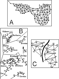
Moreover, the introduction of neighbouring relationships in the multivariate analysis of spatial structures has several advantages. Mainly, it allows various conditions of use (Figure 1).
Figure 1. Three examples of use of neighboring relationships in spatial analysis of ecological data. 1A: neighboring relationship deduced from the Delaunay triangulation of the sampling space; two point are neighbors if their corresponding Voronoi polygons have at least one side in common. 1B: simple linear relationship in a river system; only successive sampling sites along the same stream are neighbors. 1C: neighboring relationship with a geographical barrier blocking the passage between two sets of sites.
a) If the sampling zone can be considered as homogeneous (Figure 1A), a simple neighbouring relationship can be easily deduced from the Delaunay triangulation of the set of sampling sites (Green and Sibson, 1977; Sibson, 1980, see examples of use in Upton and Fingleton, 1985 or Pigliucci and Barbujani, 1991). By definition, two points are neighbours if their corresponding Voronoï polygons have at least one side in common.
b) In the case of studies in river systems (Figure 1B) neighbouring relationships are the only possible way since the spatial coordinates (x, y) of sampling sites have nearly no meaning, while upstream-downstream site positions are directly translatable into a linear neighbouring relationship (only successive sampling sites along the same stream are neighbours).
c) Neighbouring relationships are also a convenient way to take into account obstacles between sites separated by a small geographical distance (case of a geographical barrier blocking the passage between two sets of sites, Figure 1C).
In this paper, we first present the concepts of total variance, local variance, and global variability. Then, we define the multivariate analyses whose row scores maximise these quantities. We apply these methods to a simulated data set to test their ability to detect known a priori spatial structures. We also use them on an ecological data set to show the results obtained in real situations.
 is the n by p matrix containing the data (p variables
measured at n sampling sites).
is the n by p matrix containing the data (p variables
measured at n sampling sites).
 is the transpose of X.
 is a vector with components
 (e.g., any column vector from X).
 is the symmetric n by n matrix of the between-sites neighbouring
graph: if site i is neighbouring site j then
is the symmetric n by n matrix of the between-sites neighbouring
graph: if site i is neighbouring site j then
 ,
else
,
else
 .
Moreover for any i,
.
Moreover for any i,
 .
.
Matrix
 is simply deduced from M by
 ,
where m is the total number of pairs of neighbours, therefore
,
where m is the total number of pairs of neighbours, therefore
 .
.
 is the diagonal matrix of neighbouring weights:
 .
.
The mean of variable x given the weights D is equal to:
 .
(1)
.
(1)
Its variance is equal to what we call the total variance:
 .
(2)
.
(2)
If x is D-centred (i.e., if the mean of x given the weights D is equal to zero), it can be written in matrix form as:
 .
(3)
.
(3)
The local variance (Lebart, 1969; Banet and Lebart, 1984) is:
 (4)
(4)
and can be written as:
 .
(5)
.
(5)
The global variability (or spatial auto-covariance) is defined by:
 ,
(6)
,
(6)
which, if x is D-centred, can be written:
 .
(7)
.
(7)
Since it is not always positive, it cannot be called global variance. The
second form in equations (5) and (7) shows that the global variability can be
seen as the covariance between
 (the observed values) and the mean of its neighbours (7), and that the local
variance can be seen as the covariance between
(the observed values) and the mean of its neighbours (7), and that the local
variance can be seen as the covariance between
 and the difference between each point and the mean of its neighbours (5). From
equations (3), (5) and (7), we can derive a variance decomposition of the
form:
and the difference between each point and the mean of its neighbours (5). From
equations (3), (5) and (7), we can derive a variance decomposition of the
form:
 (8)
(8)
hence a decomposition of the total variability into local and global components with respect to the neighbouring relationship between observations. With a different goal, Faraj (1993) also uses neighbouring weights.
When the neighbouring weights (D) are uniform, (

 ;
this is the case for example in circular linear neighbouring relationships),
the ratio of the local variance to the total variance
;
this is the case for example in circular linear neighbouring relationships),
the ratio of the local variance to the total variance
 is equal (except a
 factor) to Geary's coefficient of autocorrelation, from which Geary's index can
be deduced (Geary, 1954; Cliff and Ord, 1973).
factor) to Geary's coefficient of autocorrelation, from which Geary's index can
be deduced (Geary, 1954; Cliff and Ord, 1973).
Similarly, we can note that Moran's index, I (Moran, 1948; Cliff and Ord, 1973;
Ripley, 1981) is exactly, under the same hypothesis, the ratio of the global
variance to the total variance
 .
.
The total, local and global multivariate analyses that maximise the
corresponding variances will be presented in the general form of the analysis
of a statistical triplet. A triplet (X, C, R) consists of
three matrices: the data matrix X (possibly after an appropriate
transformation, like centring or standardisation), the matrix of row weights
(R), and the matrix of the metric used to measure the distances between
rows (C). Reciprocally, C can also be seen as the matrix of
column weights, and R as the matrix of the metric used to measure the
distances between columns. The analysis of this statistical triplet is based on
the eigenvector analysis of matrix
 .
When
.
When
 is not proportional to the identity, this matrix is not symmetric, but the
eigenequation can be written as:
is not proportional to the identity, this matrix is not symmetric, but the
eigenequation can be written as:
 (9)
(9)
with eigenvectors
 and
and
 verifying
 .
The principal axes and the row scores are respectively
.
The principal axes and the row scores are respectively
 and
and
 .
.
See Caillez and Pagès (1976), Escoufier (1987), and Dolédec and Chessel (1994) for a general presentation of this point of view.
The usual PCA is the analysis of the triplet (
 ,
,
 ,
,

 )
where
)
where
 is the
 identity matrix,
 is the
 identity matrix and
 is the
 centred (PCA on covariance matrix) or standardised (PCA on correlation matrix)
data matrix. The row scores of this analysis maximise the usual variance.
centred (PCA on covariance matrix) or standardised (PCA on correlation matrix)
data matrix. The row scores of this analysis maximise the usual variance.
The analysis of the total structure is the analysis of the triplet (
 ,
,
 ,
D) where
,
D) where
 is the D-centred (or D-standardised) data matrix. The row scores
of this analysis maximise the total variance.
is the D-centred (or D-standardised) data matrix. The row scores
of this analysis maximise the total variance.
Following Le Foll's approach (Le Foll, 1982), the analysis of the local
structure of the data matrix can be accomplished by the analysis of the triplet (
 ,
,
 ,
,
 ).
The row scores of this analysis maximise the local variance.
).
The row scores of this analysis maximise the local variance.
Wartenberg (1985b) has presented a method called Multivariate Spatial
Correlation Analysis (MSCA), based on the eigenvector analysis of matrix
 (the
spatial covariance matrix). By introducing the D-centring and using
(the
spatial covariance matrix). By introducing the D-centring and using
 ,
we simply obtain the analysis of the global structure of the data table by the
PCA of the triplet (
,
we simply obtain the analysis of the global structure of the data table by the
PCA of the triplet (
 ,
,
 ,
P). The row scores of this analysis have the highest possible global
variability. The corresponding eigenvalues are not always positive, as they are
not variances but spatial auto-covariances (6). This does not raise any problem
in the interpretation of the analysis: a negative value just means that a high
positive value at one point is likely to be surrounded by high negative values
at neighbouring points (i.e., there is a negative spatial
auto-covariance).
,
P). The row scores of this analysis have the highest possible global
variability. The corresponding eigenvalues are not always positive, as they are
not variances but spatial auto-covariances (6). This does not raise any problem
in the interpretation of the analysis: a negative value just means that a high
positive value at one point is likely to be surrounded by high negative values
at neighbouring points (i.e., there is a negative spatial
auto-covariance).
Thanks to the D-centring, the operators of these three analyses are linked, thus providing a canonical decomposition of the total variance:
 .
(10)
.
(10)
Compared to the method proposed by Solow (1994) for extracting a common trend from a time series, our global analysis extends the concept of time trend to space trend (in fact, to any neighbouring relationship), and provides the numerical stability needed when there are many variables.
The above PCAs can be extended to Correspondence Analysis (CA). The only problem is the fact that the row weights must in this case be taken as the neighbouring weights instead of the usual CA weights, leading thus to a modified CA.
Let us first define the usual CA as the analysis of a triplet (Escoufier,
1982). Let
 be the total sum of data matrix X (containing species counts in this
case):
be the total sum of data matrix X (containing species counts in this
case):
 (11)
(11)
and let
 be the frequency matrix:
 (12)
(12)
 .
(13)
.
(13)
 and
and
 are the diagonal matrices containing the row and column frequencies:
 (14)
(14)
 .
(15)
.
(15)
With these notations, the usual CA is the analysis of the triplet (
 ,
,
 ,
,
 ).
).
 is the
 matrix with all elements equal to one. The general term
 of matrix
 is:
is:
 (16)
(16)
We can now define the total, local and global CA as being triplet analyses.
 is the diagonal matrix containing the column weights deduced from the
neighbouring relationship:
is the diagonal matrix containing the column weights deduced from the
neighbouring relationship:
 (17)
(17)
The total CA is the analysis of the triplet (
 ,
,  , D).
The local CA is the analysis of the triplet (
, D).
The local CA is the analysis of the triplet (
 ,
,  ,
,  ),
and the global CA is the analysis of the triplet (
),
and the global CA is the analysis of the triplet (
 ,
,  , P).
These CA are linked in the same way as (10). They provide
, P).
These CA are linked in the same way as (10). They provide
 -standardised
species codes which, by averaging, give in turn sample codes that maximise the
total variance, the local variance, or the global variability.
-standardised
species codes which, by averaging, give in turn sample codes that maximise the
total variance, the local variance, or the global variability.
A single set of simulated data was used to test the ability of these methods to detect total, local and global structures. This set was made of one table with seven columns, denoted x1 to x7, and 49 rows corresponding to 49 sampling sites located at the nodes of a 7x7 square grid. The values of variables x1 to x5 are sampled from a normal distribution N (0, 1) with a fixed correlation structure (table 1).
Table 1. Correlation matrix of the first five variables included in the simulated data set.
        X1         X2         X3         X4         X5
  X1    +1.00      +0.49      -0.12      +0.01      +0.23
  X2    -0.49      +1.00      +0.32      +0.25      -0.15
  X3    -0.12      +0.32      +1.00      +0.31      -0.07
  X4    +0.01      +0.25      +0.31      +1.00      +0.08
  X5    +0.23      -0.15      -0.07      +0.08      +1.00
These variables introduce structures without spatial component in the data set. Variable x6 has a fixed spatial repartition on the grid, with a maximum equal to 4 at the centre of the grid and values decreasing to 1 towards the edges. A random noise was added to this structure at each node of the grid by means of values sampled from N (0, 1). This variable presents a strong global structure. Variable x7 was built starting from 49 alternating values equal to -1 or +1, to which a normal N (0, 1) noise was also added. This variable thus presents a strong local structure. Figure 2 shows the spatial distribution of the seven variables.
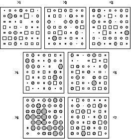
Figure 2. Graphical display of the simulated data set (x1, ..., x7) used to test the ability of the three methods to detect local and global structures. The diameter of circles and the side of squares are proportional to the values represented (circles for positive values and squares for negative ones). Variables (x1, ..., x5) are sampled from a normal distribution N (0, 1) with a fixed correlation structure (table 1). Variables x6 and x7 are built to exhibit strong global and local structures respectively (see text).
The neighbouring relationship chosen to perform the total, local and global analyses was the simple chess rook relationship with lag one. Figure 3 shows the spatial distribution of the row scores on the first axis of each analysis. It is very clear that the global structure created by variable 6 is revealed only by the first factor of global analysis, and not by total and local analyses. Conversely, the local structure of variable 7 is detected by the local analysis, and not by total and global analyses.
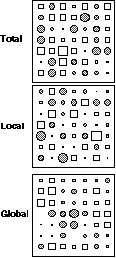
Figure 3. Row scores of the simulated data set on the first axis of total, local and global analyses. The diameter of circles and the side of squares are proportional to the values represented (circles for positive values and squares for negative ones). Local analysis detects the local structure and global analysis detects the global structure. Total analysis only reflects the non-spatial correlation structure introduced by x1, ..., x5.
Variable 6 has the highest global variability (0.17) and the smallest local variance (0.82) of all the variables, while variable 7 has the smallest global variability (-0.68) and the highest local variance (1.68). Comparatively, the first factor score of the global analysis has a global variability equal to 0.56 (the first eigenvalue of global analysis) and a local variance equal to 0.80. The first factor score of the local analysis has a local variance equal to 2.11 (the first eigenvalue of local analysis) and a global variability equal to -0.61.
The data table has 90 rows and 64 columns and contains the abundance of 64 bird
species in 90 samples (Bournaud, 1987). This table is available at the
following URL (Uniform Resource Locator):
ftp://biom3.univ-lyon1.fr/pub/datasets/EES95/tab.txt
The samples come from a zone surrounding the Rhône river near Lyon,
France; they are roughly regularly spaced. The spatial position of the 90
samples on a geographical map is given in Figure 4A.
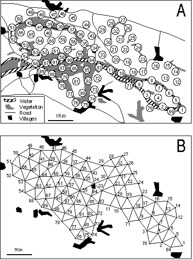
Figure 4. Geographical map of the study site (A) and the neighboring relationship deduced from the Delaunay triangulation of the set of samples (B).
This map was digitised and the XYZ GeoBench package for Macintosh micro-computers (Schorn, 1991; URL ftp://ftp.inf.ethz.ch/pub/xyz/) was used to obtain the Voronoï diagram and the corresponding Delaunay triangulation. The neighbouring relationship between samples was directly deduced from this triangulation (Figure 4B). The distribution of the 64 bird species is shown in Figure 5, where different types of distributions are clearly present (e.g., species 19 and 28).
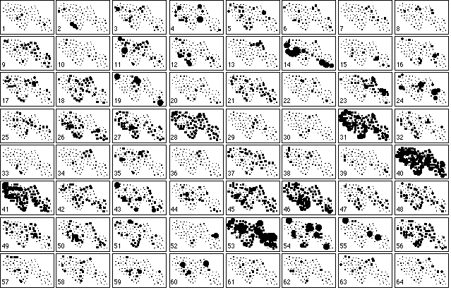
Figure 5. Collection of the 64 maps of bird species abundance in the 90 samples. Circle size is proportional to the abundance of each species. A dot denotes the absence of the species.
Figure 6 shows a representation of the first factor of the total (6A), global (6B) and local (6C) correspondence analysis on the geographical map. The circle and square sizes are proportional to sample factor scores. The contour curves are computed by a bi-dimensional lowess regression (Cleveland, 1979) over the nine nearest neighbours. Nine neighbours were chosen after looking at the variations of the smoothing error (sum of the squared differences between observed and estimated values) as a function of the number of neighbours (Figures 6A', 6B', and 6C'). See Cleveland and Devlin (1988) for a detailed explanation of this procedure. The error clearly drops for six neighbours in total and local analyses, while the minimum is only obtained for nine neighbours in the case of the global analysis. The bar charts of eigenvalues are given in Figures 6A'', 6B'', and 6C''.
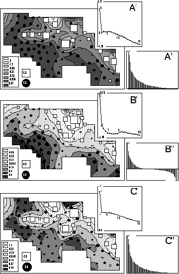
Figure 6. Map of the first factor score of total (A), global (B) and local (C) analyses. Circle and square sizes are proportional to the factor scores. Circles indicate positive values and squares negative ones. Graphs A', B' and C' show the smoothing error (sum of the squared differences between observed and estimated values) plotted against the number of neigbors used to compute the contour curves. This is a simplified version of the "M plot" technique (Cleveland and Devlin, 1988) to choose the number of neigbors in a locally weighted regression. Graphs A'', B'' and C'' represent the eigenvalues of each analysis.
The contour curves in Figure 6B show that the first factor of the global analysis is smooth, with a south-west to north-east gradient. This is consistent with the constraints put on these scores, and with the fact that nine neighbours (instead of six) where needed to achieve a satisfying smoothing. Moreover, the smoothing error is always smaller for the global analysis than for the total and local ones (Figures 6A', 6B', and 6C'). For example, with 5 neighbours, the smoothing error is equal to 0.72 for the global analysis, 1.3 for the total analysis and 1.7 for the local analysis. The observed gradient corresponds to an open/closed vegetation gradient in the sampling zone that clearly affects bird distribution.
The contour curves in Figure 6C are much less smooth than in Figure 6B. The squares and circles representation underlines the opposition between a few points showing large squares surrounded by circles. These local structures also correspond to vegetation structures (clearing and surrounding skirts) affecting bird distribution. This feature is also consistent with the fact that these scores maximise the local variance (see paragraph 3.3).
Interestingly enough, the total CA (which is just an ordinary CA with special row weights) is an intermediate between the local and global analyses (Figure 6A). The features of both constrained analyses can be found in the map of factor scores (6A), but they are obviously less clear. The open/closed gradient is hardly visible, and the opposition between circles and squares is lessened. The smoothing error decrease (6A') and the eigenvalue (6A'') charts are more like the local analysis diagrams than like the global ones. In the unconstrained analysis, the global structures are hidden by the local ones because they are forced into the same scale.
This example underlines the importance of graphical representations in the study of spatial structures in ecology. We quite agree with Birks and Myers in their discussion of the paper by Borcard and Legendre (Borcard and Legendre, 1994) on the fact that contouring and interpolation techniques should be combined with ordination methods to provide effective displays of ecological patterns. In the present work, local regression, carefully applied with the help of the smoothing error chart, shows up as a simple and efficient method for computing contour curves of factor scores.
In the comparison of the three types of analyses (total, global and local) on several ecological data sets, at least two simple situations can be distinguished, namely:
1) Total structures = global structures = local structures. This is the case if all structures are pure gradients, and the resulting interpretations are then made in terms of ordinations.
2) Total structures = global structures != local structures. This means that the structures correspond to partitions.
Moreover, as it is the case in this paper, both kinds of structures may be present simultaneously and interact (the local structures being nested in the global one).
The methods described here take into account the neighbouring relationship through the weighting of the units (with the neighbouring weights), and through the graph matrix for global and local analyses. The weighting (and the corresponding D-centring), on the one hand grants a higher importance to points having a lot of neighbours (thus lessening the importance of edge points), and on the other hand allows a unification of several points of view, mainly the introduction of Geary's and Moran's indices into multivariate analysis, and the propositions made by Lebart, 1969; Le Foll, 1982; Wartenberg, 1985b.
Neighbouring relationships also provides an alternative to the use of
orthogonal polynomials to model the spatial components of the data set. As
pointed out by Borcard and Legendre (1994, p.59), "The terms of the spatial
polynomials originally proposed by Legendre (1990) are not independent of one
another. If the interpretation of the regression or canonical coefficients
relating these terms to the community structure is of special interest,
orthogonal polynomials should be used instead of the classical polynomials".
The eigenvectors of the so-called smoothing operators
 and
and
 (that arise in equations 5 and 7) are the same, and they define a
 -
orthonormal
basis on which the data can be projected to obtain a decomposition of the
global phenomenon.
-
orthonormal
basis on which the data can be projected to obtain a decomposition of the
global phenomenon.

Figure 7. Graphical display of the first six eigenvectors of the smoothing operators. Circles and squares (A) are best to show partitions of the area, while contour curves (C) underline the smoothness of the phenomenon. Grey level polygons (B) seem less effective. The graph of the smoothing error (D) can be used to determine the number of neighbors neeeded to compute contour curves; here 5 neighbors are enough.
Figure 7 shows three representations of the first six eigenvectors of the smoothing operator associated to the neighbouring relationship in our example. Figure 7A is drawn with circles and squares, Figure 7B with grey level polygons, and Figure 7C with contour curves. Grey level polygons are probably the worst type of representation. Contour curves underline the smoothness of the eigenvectors, while circles and squares stress the cutting out of spatial patterns. The graph of the variations of the smoothing error for contour curves (Figure 7D) shows that this error increases with the rank of the eigenvector (curve 1 to 6), and with the number of neighbours when it is greater than 5 or 6.
The problem of modelling the non spatially structured fractions (Borcard and Legendre, 1994 p. 60) can also be tackled by using the last (instead of the first) eigenvectors of the smoothing operators. Indeed, these eigenvectors are "anti-smooth" and thus provide a good way to model local structures.
The use of neighbouring relationships is very general and can be extended to other types of analyses. This has been demonstrated here for Correspondence Analysis, but it is also applicable to Multiple Correspondence Analysis (in the case of qualitative variables) for example. It is also particularly interesting in methods for relating two data tables to one another, and we are preparing a follow-up to this paper dealing with the introduction of neighbouring relationships in co-inertia analysis (Chessel and Mercier, 1993; Dolédec and Chessel, 1994), and in the family of instrumental variable analyses, like CCA (Ter Braak, 1986) and the PLS (partial least square) or WA-PLS (weighted averaging partial least square) regressions (Ter Braak et al., 1993).
The computer programs used to perform the computations and graphical displays shown here are part of the ADE package (Chessel and Dolédec, 1993; Thioulouse et al., 1995). This package, for Apple Macintosh micro-computers, is freely available on the Internet at the following URL:
ftp://biom3.univ-lyon1.fr/pub/mac/ADE/ADE4/
or through this WWW (World Wide Web) page:
http://biomserv.univ-lyon1.fr/ADE-4.html
Acknowledgements
We wish to thank C.J.F. ter Braak and another reviewer, whose helpful comments and suggestions have allowed us to greatly improve the first version of this text.
References
Banet, T.A. and Lebart, L. (1984). Local and partial principal components analysis (PCA) and correspondence analysis (CA). In COMPSTAT 84. International Association for Statistical Computing (eds), Physica-Verlag, Vienna, Austria. pp. 113-123.
Borcard, D., Legendre, P., and Drapeau, P. (1992). Partialling out the spatial component of ecological variation. Ecology, 73, 1045-1055.
Borcard, D. and Legendre, P. (1994). Environmental control and spatial structure in ecological communities: an example using oribatid mites (Acari, Oribatei). Environmental and Ecological Statistics, 1, 37-61.
Bournaud, M. (1990). Peuplement d'oiseaux et propriétés des écocomplexes de la plaine du Rhône: descripteurs de fonctionnement global et gestion des berges. Rapport sur programme SRETIE, Ministère de l'Environnement, pp. 1-135.
Cailliez, F. and Pages, J.P. (1976). Introduction à l'analyse des données. SMASH, Paris, France.
Chessel, D. and Dolédec, D. (1993). ADE software. Multivariate analyses and graphical display for environmental data. Version 3.7. User manual (in French), 8 sections, 750 pages. URA CNRS 1451, Université de Lyon 1, 69622 Villeurbanne CEDEX, France.
Chessel, D. and Mercier, P. (1993). Couplage de triplets statistiques et liaisons espèces-environnement. In Biométrie et Environnement, J.D. Lebreton and B. Asselain (eds), Masson, Paris, France. pp. 15-44.
Cleveland, W.S. (1979). Robust locally weighted regression and smoothing scatterplots. Journal of the American Statistical Association, 74, 829-836.
Cleveland, W.S. and Devlin, S.J. (1988). Locally weighted regression: an approach to regression analysis by local fitting. Journal of the American Statistical Association, 83, 596-610.
Cliff, A.D. and Ord, J.K. (1973). Spatial autocorrelation. Pion, London, England.
Dolédec, S. and Chessel, D. (1994). Co-inertia analysis: an alternative method for studying species-environment relationships. Freshwater Biology, 31, 277-294.
Escoufier, Y. (1982). L'analyse des tableaux de contingence simples et multiples. Metron, 40, 53-77.
Escoufier, Y. (1987). The duality diagram: a means for better practical applications. In Developments in numerical ecology, P. Legendre and L. Legendre (eds), NATO Advanced Study Institute, Series G (Ecological Sciences). Springer Verlag, Berlin, Germany. pp. 139-156.
Faraj, A. (1993). Analyse de contiguité: une analyse discriminante généralisée à plusieurs variables qualitatives. Revue de Statistique Appliquée, 41, 73-84.
Geary, R.C. (1954). The contiguity ratio and statistical mapping. The Incorporated Statistician, 5, 115-145.
Gittins, R. (1968). Trend surface analysis of ecological data. J. Ecol., 56, 845-869.
Green, P.J. and Sibson, R. (1977). Computing Dirichlet tesselations in the plane. The Computer Journal, 21, 168-173.
Lebart, L. (1969). Analyse statistique de la contiguïté. Publication de l'Institut de Statistiques de l'Université de Paris, 28, 81-112.
Lee, P.J. (1969). Theory and application of canonical trend surface analysis. Journal of Geology, 77, 303-318.
Lee, P.J. (1981). The most predictable surface (MPS) mapping method in Petroleum exploration. Bulletin of Canadian Petroleum Geology, 29, 224-240.
Le Foll, Y. (1982). Pondération des distances en analyse factorielle. Statistiques et Analyse des Données, 7, 13-31.
Legendre, P. (1993). Spatial autocorrelation: trouble or new paradigm ? Ecology, 74, 1659-1673.
Moran, P.A.P. (1948). The interpretation of statistical maps. Journal of the Royal Statistical Society B, 10, 243-251.
Pigliucci, M. and Barbujani, G. (1991). Geographical patterns of gene frequencies in Italian populations of Ornithogalum montanun (Liliaceae). Genetical Research, Cambridge, 58, 95-104.
Ripley, B.D. (1981). Spatial statistics. John Wiley, New York, USA.
Schorn, P. (1991). Implementing the XYZ GeoBench: A programming environment for geometric algorithms. In Computational Geometry: Methods, Algorithms and Applications, H. Bieri and H. Noltemeier (eds), Proc. CG'91, International Workshop on Computational Geometry, Bern, March 1991, Springer LNCS 553, pp. 187-202.
Sibson, R. (1980). The Dirichlet tesselation as an aid in data analysis. Scandinavian Journal of Statistics, 7, 14-20.
Solow, A.R. (1994). Detecting change in the composition of a multispecies community. Biometrics, 50, 556-565.
ter Braak, C.J.F. (1986). Canonical correspondence analysis: a new eigenvector method for multivariate direct gradient analysis. Ecology, 67, 1167-1179.
ter Braak, C.J.F., Juggins, S., Birks, H.J.B., and Van der Voet, H. (1993). Weighted averaging partial least squares regression (WA-PLS): definition and comparison with other methods for species-environment calibration. In Multivariate Environmental Statistics, G.P. Patil and C.R. Rao (eds), North Holland, Amsterdam, pp. 525-560.
Thioulouse J., Dolédec S., Chessel D., and Olivier J.M. (1995). ADE software: multivariate analysis and graphical display of environmental data. In Software per l'ambiente, G. Guariso and A. Rizzoli (Eds), Pàtron editore, Bologne, pp. 57-62.
Upton, G.J.G., and Fingleton, B. (1985). Spatial data analysis by example. Volume 1: Point pattern and quantitative data. Wiley, Chichester, England.
van den Wollenberg, A.L. (1977). Redundancy analysis. An alternative for canonical correlation analysis. Psychometrika, 42, 207-219.
Wartenberg, D. (1985a). Canonical trend surface analysis: a method for describing geographic patterns. Systematic Zoology, 34, 259-279.
Wartenberg, D. (1985b). Multivariate spatial correlation: a method for exploratory geographical analysis. Geographical Analysis, 17, 263-283.