Jean Thioulouse (1), Daniel Chessel (2), Sylvain Dolédec (2) & Jean-Michel Olivier (2)
(1) Laboratoire de Biométrie, Génétique et Biologie des Populations, UMR CNRS 5558, Université Lyon 1, 69622 Villeurbanne Cedex, France.
(2) Laboratoire d'Ecologie des Eaux Douces et des Grands Fleuves, URA CNRS 1974, Université Lyon 1, 69622 Villeurbanne Cedex, France.
Note : A PDF version of this paper available here : pdf, and a list of citations is available here : references.
2. The user interface
2.1 Computational modules
2.2 Graphical modules
2.3 HyperCard and WinPlus interface
3. Data analysis methods
3.1 One table methods
3.2 One table with spatial structures
3.3 One table with groups of rows
3.4 Linear regression
3.5 Two-tables coupling methods
3.6 Coinertia analysis method
3.7 K-table analysis methods
4. Graphical representations
4.1 One dimensional graphics
4.2 Curves
4.3 Scatters
4.4 Cartography modules
Availability
Acknowledgements
References
We present ADE-4, a multivariate analysis and graphical display software. Multivariate analysis methods available in ADE-4 include usual one-table methods like principal component analysis and correspondence analysis, spatial data analysis methods (using a total variance decomposition into local and global components, analogous to Moran and Geary indices), discriminant analysis and within/between groups analyses, many linear regression methods including lowess and polynomial regression, multiple and PLS (partial least squares) regression and orthogonal regression (principal component regression), projection methods like principal component analysis on instrumental variables, canonical correspondence analysis and many other variants, coinertia analysis and the RLQ method, and several three-way table (k-table) analysis methods. Graphical display techniques include an automatic collection of elementary graphics corresponding to groups of rows or to columns in the data table, thus providing a very efficient way for automatic k-table graphics and geographical mapping options. A dynamic graphic module allows interactive operations like searching, zooming, selection of points, and display of data values on factor maps. The user interface is simple and homogeneous among all the programs; this contributes to make the use of ADE-4 very easy for non specialists in statistics, data analysis or computer science.
Key words:
Multivariate analysis, principal component analysis, correspondence analysis, instrumental variables, canonical correspondence analysis, partial least squares regression, coinertia analysis, graphics, multivariate graphics, interactive graphics, Macintosh, HyperCard, Windows 95.
Corresponding author:
Jean Thioulouse
Laboratoire de Biométrie - Université Lyon 1
69622 Villeurbanne Cedex - France
ADE-4 is a multivariate analysis and graphical display software for Apple Macintosh and Windows 95 microcomputers. It is made of several stand-alone applications, called modules, that feature a wide range of multivariate analysis methods, from simple one-table analysis to three-way table analysis and two-table coupling methods. It also provides many possibilities for helpful graphical display in the process of analyzing multivariate data sets. It has been developed in the context of environmental data analysis, but can be used in other scientific disciplines (e.g., sociology, chemometry, geosciences, etc.), where data analysis is frequently used. It is freely available on the Internet network. Here, we wish to present the main characteristics of ADE-4, from three point of view: (1) user interface, (2) data analysis methods, and (3) graphical display capabilities.
ADE-4 is made of a series of small independent modules that can be used independently from each other or launched through a HyperCard interface. There are two categories of modules: computational modules and graphical ones, with a slightly different user interface.
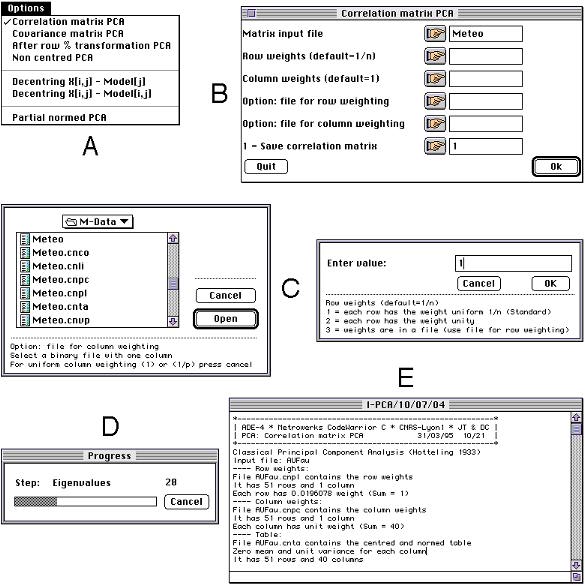
Computational modules present an "Options" menu that enables the user to choose between the possibilities available in the module. For example, in the PCA (principal component analysis) module, it is possible to choose between PCA on correlation or on covariance matrix (Figure 1A).
Fig. 1. Elements of the user interface of computational modules. A: the Options menu serves to choose the desired method. B: the main dialog window allows the user to type in the parameters of the analysis (data file name, weighting options, etc.). When the user clicks on the hand icon buttons, special dialog windows (C) make easier the selection of these parameters. During time consuming operations (e.g., computation of the eigenvalues and eigenvectors of large matrices), a progress window (D) shows the state of the program. At the end of computations, a text report is generated (E) displaying the results of the analysis.
According to the option selected by the user, a dialog window is displayed, showing the parameters required for the execution of the analysis (Figure 1B). The user can click on the buttons with a hand icon to set the values of these parameters through standard dialog windows (Figure 1C). The OK button starts the computations, and the Quit button quits the module. A progress window shows the computation steps while the analysis is being performed (Figure 1D), and a text report that contains a description of input and output files and of analysis results is created (Figure 1E).
Graphical modules also present an "Options" menu to choose the type of graphic. They have an additional "Windows" menu (Figure 2A). This menu can be used to choose one of the three parameter windows that allow an interactive definition of the graphical parameters. The user can thus freely modify the values of all the parameters and the resulting graphic is displayed in the "Graphics" window.
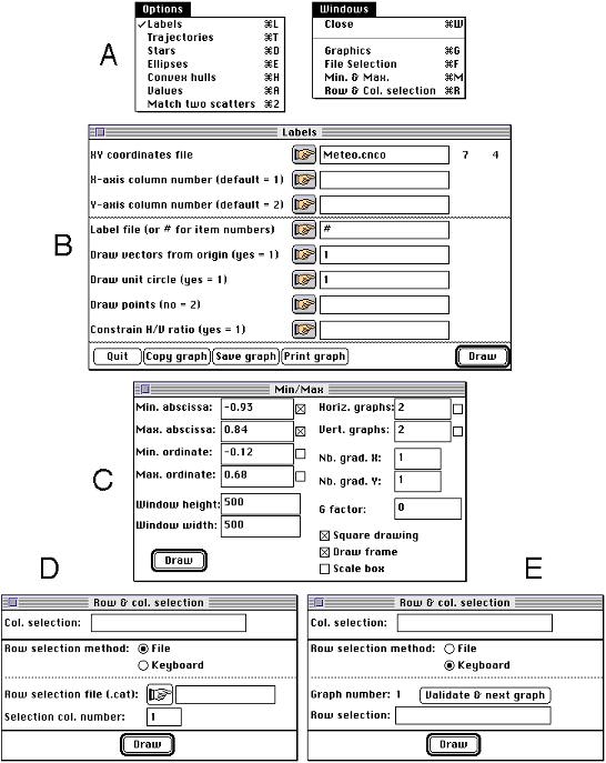
Fig. 2. Elements of the user interface of graphical modules. A: the Options menu serves to choose the type graphic, and the Windows menu can be used to choose one of the three parameter windows (B, C, D and E). The main dialog window (B) works in the same way as in computation modules. The "Min/Max" window (C) allows to set the value of numerous graphic parameters, particularly the minimum and maximum of abscissas and ordinates, the number of horizontal and vertical graphics (for graphic collections), the graphical window width and height, legend scale options, etc. The "Row & Col. selection" window (D and E) has two states (File and Keyboard), corresponding to the way of entering the selection of rows making a collection of graphics. In the File state (D), the user can choose a file containing the qualitative variable which categories define the groups of rows, and in the Keyboard (D) state, he must type in the numbers of the rows belonging to each elementary graphic.
The main dialog window (Figure 2B) allows to choose the input file and related parameters. The Copy, Save and Print buttons perform the corresponding actions on the graphic currently displayed in the "Graphics" window. The Draw button triggers the drawing, and the Quit button quits the module. In the "Min/Max" window (Figure 2C), the user can set the values of the minimum and maximum of abscissas and ordinates, the number of horizontal and vertical graphics (for graphic collections), the graphical window width and height, legend scale options, etc. In the "Row & Col. selection" (Figure 2D and 2E) window, he can choose the columns and the rows of the data set that will be used to make each elementary graphic of a collection. The rows can be chosen either through a selection file containing a qualitative variable which modalities define the groups corresponding to each graphic (Figure 2D), or by typing the number of the rows belonging to each group (Figure 2E).
2.3 HyperCard and WinPlus interface
A HyperCard (Macintosh version) or WinPlus (Windows 95 version) stack (ADE*Base) can be used to launch the modules. This stack also displays the files that are in the current data folder, and provides a way to navigate through two other stacks: ADE*Data, and ADE*Biblio.
ADE*Data is a library of c. 150 example data sets of varying size that can be used for trial runs of data analysis methods. Most of these data sets come from environmental studies. ADE*Biblio is a bibliography stack with more than 800 bibliographic references on the statistical methods and data sets available in ADE-4.
The data analysis methods available in ADE-4 will not be presented here, due to lack of space. They are based on the duality diagram (Cailliez and Pagès, 1976; Escoufier 1987). In many modules, Monte-Carlo tests (Good 1993, chapter 13) are available to study the significance of observed structures.
Three basic multivariate analysis methods can be applied to one-table data sets (Dolédec and Chessel, 1991). The corresponding modules are the PCA (principal components analysis) module for quantitative variables, the COA (correspondence analysis) module for contingency tables (Greenacre, 1984), and the MCA (multiple correspondence analysis) module for qualitative (discrete) variables (Nishisato, 1980; Tenenhaus and Young, 1985). A fourth module, HTA (homogeneous table analysis) is intended for homogeneous tables, i.e., tables in which all the values come from the same variable (for example, a toxicity table containing the toxicity of some chemical compounds toward several animal species, see Devillers and Chessel, 1995).
The DDUtil (duality diagram utilities) module provides several interpretation helps that can be used with any of the methods available in the first four modules, namely: biplot representation (Gabriel 1971, 1981), inertia analysis for rows and columns (particularly for COA, see Greenacre 1984), supplementary rows and/or columns (Lebart et al., 1984), and data reconstitution (Lebart et al., 1984).
The PCA module offers several options, corresponding to different duality diagrams: correlation matrix PCA, covariance matrix PCA, non centered PCA (Noy-Meir, 1973), decentered PCA, partially standardized PCA (Bouroche, 1975), within-groups standardized PCA (Dolédec and Chessel, 1987). See Okamoto (1972) for a discussion of different types of PCA.
The COA module offers six options for correspondence analysis (CA): classical CA, reciprocal scaling (Thioulouse and Chessel, 1992), row weighted CA, internal CA (Cazes et al., 1988), decentered CA (Dolédec et al., 1995).
The MCA module offers two options for the analysis of tables made of qualitative variables: Multiple Correspondence Analysis (Tenenhaus and Young, 1985) and Fuzzy Correspondence Analysis (Chevenet et al., 1994; Castella and Speight, 1996).
3.2 One table with spatial structures
Environmental data very often include spatial information (e.g., the spatial location of sampling sites), and this information is difficult to introduce in classical multivariate analysis methods. The Distances module provides a way to achieve this, by using a neighboring relationship between sites. See Lebart (1969) for a presentation of this approach and Thioulouse et al. (1995) for a general framework based on variance decomposition formulas. Also available in this module are the Mantel test (Mantel, 1967), the principal coordinate analysis (Manly, 1994), and the minimum spanning tree (Kevin and Whitney, 1972).
3.3 One table with groups of rows
When a priori groups of individuals exist in the data table, the Discrimin module can be used to perform a discriminant analysis (DA, also called canonical variate analysis), and between-groups or within-groups analyses (Dolédec and Chessel, 1989).. These three methods can be performed after a PCA, a COA, or an MCA, leading to a great variety of analyses. For example, in the case of DA, we can obtain after a PCA, the classical DA (Mahalanobis, 1936, Tomassone et al., 1988), after a COA, the correspondence DA, and after an MCA the DA on qualitative variables (Saporta, 1975, Persat et al., 1985). Monte-Carlo tests are available to test the significance of the between-groups structure.
Three modules provide several linear regression methods. These modules are UniVarReg (for univariate regression), OrthoVar (for orthogonal regression), and LinearReg (for linear regression). Here also, Monte-Carlo tests are available to test the results of these methods.
The UniVarReg module deals with two regression models: polynomial regression and Lowess method (locally weighted regression and smoothing scatterplots; Cleveland 1979, Cleveland and Devlin, 1988).
The OrthoReg module performs multiple linear regression in the particular case of orthogonal explanatory variables. This is useful for example in PCR (principal component regression; Næs, 1984), or in the case of the projection on the subspace spaned by a series of eigenvectors (Thioulouse et al., 1995).
The LinearReg module performs the usual multiple linear regression (MLR), and the first generation PLS (partial least squares) regression (Lindgren, 1994). See also Geladi and Kowalski (1986); Höskuldsson (1988) for more details on PLS regression.
3.5 Two-tables coupling methods
One module is dedicated to two-tables coupling methods based on projection onto vector subsapces (Takeuchi et al., 1982). It has eleven options that perform complex operations. The first six options allow to build orthonormal bases on which the projections can be made. The last five options provide several two-tables coupling methods, and mainly PCAIV (PCA on Instrumental Variables) methods. The "PCA on Instrumental Variables" option can be used with any statistical triplet from the PCA, COA and MCA modules, which corresponds for example to methods like CAIV (correspondence analysis on instrumental variables, Lebreton et al., 1988a, 1988b, 1991) or CCA (canonical correspondence analysis, ter Braak, 1987a, 1987b).
There are two modules for coinertia analysis. The Coinertia module, which performs the usual coinertia analysis (Chessel and Mercier, 1993; Dolédec and Chessel, 1994; Thioulouse and Lobry, 1995; Cadet et al., 1994), and the RLQ module, which performs a three-table generalization of coinertia analysis (Dolédec et al., 1996).
Collections of tables (three-ways tables, or k-tables) can be analyzed with the STATIS module that features three distinct methods: STATIS (Escoufier, 1980; Lavit 1988; Lavit et al., 1994), the partial triadic analysis (Thioulouse and Chessel, 1987), and the analysis of a series of contingency tables (Foucart, 1978). The KTabUtil module provides a series of three-ways table manipulation utilities: k-table transposition, sorting, centering, standardization, etc. Two generalisations of k-tables coinertia analysis are also available.
ADE-4 features 14 graphical modules, that fall broadly in four categories: one dimensional graphics, curves, scatters, and geographical maps. Most modules have the possibility to draw automatically collections of graphics, corresponding to the columns of the data file (one graphic for each variable), to groups of rows (one graphic for each group), or to both (one graphic for each group and for each variable). This feature is particularly useful in multivariate analysis, where one always deals with many variables and/or groups of samples. Moreover, several modules have two versions, according to the way they treat the collections: elementary graphics can be either simply put side by side, or superimposed. Superimposition is done in the modules with a name ending with the "Class" suffix.
The Graph1D module is intended for one dimensional data representation, such as the values of one factor score. It has two options: histograms and labels. The histograms option computes the distribution of the values into classes and draws the corresponding histogram, with optionally the adjusted Gauss curve superimposed over it. The Labels option simply draws regularly spaced labels (that can be chosen by the user) vertically or horizontally along an axis; these labels are connected by lines to the corresponding coordinates on the axis. The columns and groups of rows corresponding to each elementary graphic of a collection can be chosen by the user.
The Graph1DClass module is also intended for representing one dimensional data, but, as the "Class" suffix indicates, when there are groups of rows and when the corresponding graphics must be superimposed instead of placed side by side. Because superimposed histograms and labels are not convenient, this is used only for Gauss curves. Figure 3 shows an example of such graphic: each elementary graphic contains a collection of superimposed Gauss curves. Each curve corresponds to one group of rows in the data table. The successive elementary graphics correspond to several partitions of the set of rows (i.e., to several qualitative variables). All these parameters are interactively set by the user.
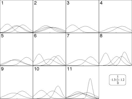
Fig. 3. Example of graphic drawn with the Graph1DClass module: the eleven elementary graphics (numbered 1 to 11) correspond to eleven qualitative variables. In each elementary graphic, the Gauss curves represent the distribution of the samples belonging to the categories of each qualitative variable. For example, graphic number seven corresponds to the seventh qualitative variable, which have two categories. The two Gauss curves represent the mean and the variance of the samples belonging to each of these two categories. Only one quantitative variable of the data table is represented here. In this module, elementary graphics of a collection corresponding to groups of rows are superimposed, while graphics corresponding to the qualitative variables are placed side by side. Graphics corresponding to other columns of the data table (quantitative variables) would also be placed side by side.
The Curves module draws curves, i.e., series of values (ordinates) that are plotted along an axis (abscissas). It features four options: Lines, Bars, Steps and Boxes. Here also, columns and groups of rows can correspond to the elementary graphics of a collection. Boxes are simply the classical "box and whiskers" display, showing the median, quartiles, minimum and maximum.
The CurveClass module acts in the same way as the Curves module, except that the curves defined by the qualitative variable are superimposed in the same elementary graphic instead of being dispatched in several graphics.
The CurveModels module allows to fit Lowess and polynomial models. This module automatically fits a model for each elementary graphic in a collection.
The most classical graphic in multivariate analysis is the factor map. The Scatters module is designed to draw such graphics, with several options. For all options, the user can interactively select the columns and the groups of rows that will be used to draw the elementary graphics that make a collection. The simplest option is Labels. For each point, it only draws a characters string (label) on the factor map (Figure 4A).
The Trajectories option underlines the fact that the elements are ordered (for example in the case of time series) by linking the points with a line (Figure 4B).
The Stars option computes the gravity center of each group of points and draws lines connecting each element to its gravity center (Figure 4C).
The Ellipses option computes the means, variances and covariance of each group of points on both axes, and draws an ellipse with these parameters: the center of the ellipse is centered on the means, its width and height are given by the variances, and the covariance sets the slope of the main axis of the ellipse (Figure 4D).
The Convex hulls option simply draws the convex hull of each set of points (Figure 4E). Ellipses and convex hulls are labeled by the number of the group.
The Values option is slightly more complex. For each point on the factor map, it draws a circle or a square which size is proportional to a series of values (circle are for positive values, and squares for negative ones). These series of values can be chosen as the columns of a separate file (Figure 4F). This technique is particularly useful to represent data values on the factor map.
Lastly, the "Match two scatters" option can be used when two sets of scores are available for the same points (this is frequently the case in co-inertia analysis and other two-table coupling methods). It draws an arrow starting from the coordinates of the point in the first set and ending at the coordinates in the second set (Figure 4G).
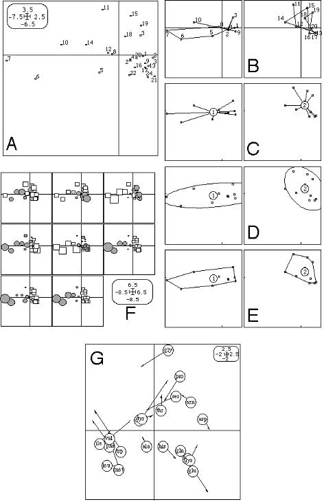
Fig. 4. Example of graphics drawn with the Scatters module: labels (A), trajectories (B), stars (C), ellipses (D), convex hulls (E), circles and squares (F: circles are for positive values, squares for negative ones), and two scatters matching (G). The coordinates of points are given by two columns chosen in a table. In this module, elementary graphics of a collection correspond to groups of rows, except for the circles and squares option, in which they can correspond to groups of rows and also to the columns of the file containing the values to which circle and square sizes are proportional (in this case, if there are k groups and p columns, the number of elementary graphics will be equal to k.p).
The ScatterClass module incorporates the Labels, Trajectories, Stars, Ellipses and Convex hulls options. It superimposes the elementary graphics corresponding to a collection. Figure 5 shows an example where eleven elementary graphics (corresponding to eleven qualitative variables) are represented. In each graphic, several convex hulls (corresponding to groups of points) are superimposed. The points themselves are not drawn.
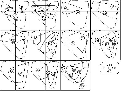
Fig. 5. Example of graphic drawn with the ScatterClass module. Like in figure 3, the eleven graphics correspond to eleven qualitative variables. The convex hulls containing the points belonging to the categories of the qualitative variable are drawn in each elementary graphic. The dots corresponding to each point have not been drawn. Like the Scatters module, ScatterClass can also draw label, trajectories, stars, and ellipses.
The last module for scatter diagrams is ADEScatters (Thioulouse, 1996). It is a dynamic graphic module, in which the user can perform several actions that help interpreting the factor map: searching, zooming, selection of sets of points, interactive display of data values on the factor map.
Four cartography modules are available in ADE-4. They can be used to map either the initial (raw or transformed) data, or the factor scores resulting from a multivariate analysis.
The Maps module has three options: the Labels option simply draws a label on the map at each sampling point, the Values option draws circles (positive values) and squares (negative values) with sizes proportional to the values of the data file, and the Neighboring graph option draws the edges of a neighboring relationship between the points.
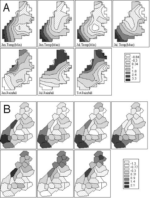
Fig. 6. Example of graphic drawn with the Levels and the Areas modules. The Levels module (A) draws contour curves with gray level patterns that indicate the curve value. The Areas module (B) draws grey level polygons on a geographical map. For both modules, collections correspond to the columns of the table containing the values displayed on the map (grey levels). Here, the seven contour curve maps and the seven grey level area maps correspond to seven columns of the data file.
The Levels module draws contour curves on the map (Figure 6A). It can be used with sampling points having any distribution on the map: an interpolated regular grid, is computed before drawing. Contour curves are computed by a lowess regression over a number of neighbors chosen by the user (see Thioulouse et al., 1995 for a description and example of use of this technique in environmental data analysis).
The Areas module draws maps with gray level polygons (Figure 6B), starting from a file containing the coordinates of the vertices of each of the areas making the map, and a second file corresponding to the gray levels.
The computing power of today micro-computers is such that the time needed to perform the computations of multivariate analysis methods is no more a limiting factor. The time needed to compute all the eigenvalues and eigenvectors of a 100 x 100 matrix is just a few seconds. The limiting factor is rather the amount of field work needed to collect the data. This fact has several consequences on multivariate analysis software packages. Monte-Carlo-like methods (permutation tests) can, and should be used much more widely (Good, 1993 p. 8). Moreover, it is possible to use an interactive approach to multivariate analysis, trying several methods in just a few minutes. But this implies an easy to use graphical user interface, particularly for graphic programs, allowing to explore many ways of displaying data structures (data values themselves or factor scores). Trend surface analysis and contour curves are valuable tools for this purpose. We also need a graphical software able to display simultaneously all the variables of the dataset, and several groups of samples, corresponding for example to the experimental design (e.g., samples coming from several regions). We have tried to address these points in ADE-4.
One of the benefits of having a systematic approach to elementary graphics collection in modules Graph1D, Graph1dClass, Curves, CurveClass, Scatters, and ScatterClass is the possibility to draw automatically all the graphics of a k-table analysis (i.e., the graphics corresponding to the analyses of all the elementary tables).
ADE-4 can be obtained freely by anonymous FTP to biom3.univ-lyon1.fr, in the /pub/mac/ADE/ADE4 directory. Previous versions (up to version 3.7) has already been distributed to many research laboratories in France and other countries. A WWW (world-wide web) documentation and downloading page is available at : http://biomserv.univ-lyon1.fr/ADE-4.html , which also provides access to updates and user support through the ADEList mailing list. A sub-set of ADE-4 can be used on line on the Internet, through a WWW user interface called NetMul (Thioulouse and Chevenet, 1996) at the following address : http://biomserv.univ-lyon1.fr/NetMul.html .
ADE-4 development was supported by the "Programme Environnement" of the French National Center for Scientific Research (CNRS), under the "Méthodes, Modèles et Théories" contract.
Bouroche, J.M. (1975). Analyse des données ternaires: la double analyse en composantes principales. Thèse de 3deg. cycle, Université de Paris VI.
Cadet, P., Thioulouse, J. and Albrecht, A. (1994). Relationships between ferrisol properties and the structure of plant parasitic nematode communities on sugarcane in Martinique (French West Indies). Acta Œcologica, 15, 767-780.
Cailliez, F. and Pages, J.P. (1976). Introduction à l'analyse des données. SMASH: Paris.
Castella, E. & Speight, M.C.D. (1996) Knowledge representation using fuzzy coded variables: an example based on the use of Syrphidae (Insecta, Diptera) in the assessment of riverine wetlands. Ecological Modelling, 85, 13-25.
Cazes, P., Chessel, D. and Dolédec, S. (1988). L'analyse des correspondances internes d'un tableau partitionné : son usage en hydrobiologie. Revue de Statistique Appliquée 36, 39-54.
Chessel, D. and Mercier, P. (1993). Couplage de triplets statistiques et liaisons espèces-environnement. In Biométrie et Environnement., Lebreton J.D. and Asselain B. (eds), 15-44. Paris: Masson.
Chevenet, F., Dolédec, S. and Chessel, D. (1994). A fuzzy coding approach for the analysis of long-term ecological data. Freshwater Biology 31, 295-309.
Cleveland, W.S. (1979). Robust locally weighted regression and smoothing scatterplots. Journal of the American Statistical Association 74, 829-836.
Cleveland, W.S. and Devlin, S.J. (1988). Locally weighted repression: an approach to regression analysis by local fitting. Journal of the American Statistical Association 83, 596-610.
Devillers, J. and Chessel, D. (1995) Can the enucleated rabbit eye test be a suitable alternative for the in vivo eye test? A chemometrical response. Toxicology Modelling, 1, 21-34.
Dolédec, S. and Chessel, D. (1987). Rythmes saisonniers et composantes stationnelles en milieu aquatique I- Description d'un plan d'observations complet par projection de variables. Acta Œcologica, Œcologia Generalis 8, 403-426.
Dolédec, S. and Chessel, D. (1989). Rythmes saisonniers et composantes stationnelles en milieu aquatique II- Prise en compte et élimination d'effets dans un tableau faunistique. Acta Œcologica, Œcologia Generalis 10, 207-232.
Dolédec, S. and Chessel, D. (1991). Recent developments in linear ordination methods for environmental sciences. Advances in Ecology, India 1, 133-155.
Dolédec, S. and Chessel, D. (1994). Co-inertia analysis: an alternative method for studying species-environment relationships. Freshwater Biology 31, 277-294.
Dolédec, S., Chessel, D., Ter Braak, C.J.F. and Champely, S. (1996). Matching species traits to environmental variables: a new three-table ordination method. Environmental and Ecological Statistics 3, 143-166.
Dolédec, S., Chessel, D. and Olivier, J.M. (1995). L'analyse des correspondances décentrée: application aux peuplements ichtyologiques du Haut-Rhône. Bulletin Français de Pêche et de Pisciculture 336, 29-40.
Escoufier, Y. (1980). L'analyse conjointe de plusieurs matrices de données. In Biométrie et Temps. Jolivet, M. (eds), 59-76. Paris: Société Française de Biométrie.
Escoufier, Y. (1987). The duality diagramm : a means of better practical applications. In: Development in numerical ecology. Legendre, P. and Legendre, L. (Eds.), 139-156. NATO advanced Institute, Serie G. Berlin: Springer Verlag.
Lavit, Ch., Escoufier, Y., Sabatier, R. and Traissac, P. (1994). The ACT (Statis method). Computational Statistics and Data Analysis 18, 97-119.
Foucart, T. (1978). Sur les suites de tableaux de contingence indexés par le temps. Statistique et Analyse des données 2, 67-84.
Gabriel, K.R. (1971). The biplot graphical display of matrices with application to principal component analysis. Biometrika 58, 453-467.
Gabriel, K.R. (1981). Biplot display of multivariate matrices for inspection of data and diagnosis. In Interpreting multivariate data. Barnett, V. (eds), 147-174. New York: John Wiley and Sons.
Geladi, P. & Kowalski, B.R. (1986). Partial least-squares regression: a tutorial. Analytica Chimica Acta, 1, 185, 19-32.
Good, P. (1993). Permutation tests. New-York: Springer-Verlag
Greenacre, M. (1984). Theory and applications of correspondence analysis. London: Academic Press.
Höskuldsson, A. (1988). PLS regression methods. Journal of Chemometrics 2, 211-228.
Kevin, V. and Whitney, M. (1972). Algorithm 422. Minimal Spanning Tree [H]. Communications of the Association for Computing Machinery 15, 273-274.
Lavit, Ch. (1988). Analyse conjointe de tableaux quantitatifs. Paris: Masson.
Lebart, L. (1969). Analyse statistique de la contiguïté. Publication de l'Institut de Statistiques de l'Université de Paris 28, 81-112.
Lebart, L., Morineau, L. and Warwick, K.M. (1984). Multivariate descriptive analysis: correspondence analysis and related techniques for large matrices. New York: John Wiley and Sons.
Lebreton, J.D., Chessel, D., Prodon, R. and Yoccoz, N. (1988). L'analyse des relations espèces-milieu par l'analyse canonique des correspondances. I. Variables de milieu quantitatives. Acta Œcologica, Œcologia Generalis 9, 53-67.
Lebreton, J.D., Richardot-Coulet, M., Chessel, D. and Yoccoz, N. (1988). L'analyse des relations espèces-milieu par l'analyse canonique des correspondances . II Variables de milieu qualitatives. Acta Œcologica, Œcologia Generalis 9, 137-151.
Lebreton, J.D., Sabatier, R., Banco, G. and Bacou, A.M. (1991). Principal component and correspondence analyses with respect to instrumental variables : an overview of their role in studies of structure-activity and species-environment relationships. In Applied Multivariate Analysis in SAR and Environmental Studies. Devillers, J. and Karcher, W. (eds), 85-114. Dordrecht: Kluwer Academic Publishers.
Lindgren, F. (1994). Third generation PLS. Some elements and applications. Research Group for Chemometrics. Department of Organic Chemistry, 1-57. Umeå: Umeå University.
Mahalanobis, P.C. (1936). On the generalized distance in statistics. Proceedings of the National Institute of Sciences of India 12, 49-55.
Manly, B.F. (1994). Multivariate Statistical Methods. A primer. London: Chapman and Hall.
Mantel, M. (1967). The detection of disease clustering and a generalized regression approach. Cancer Research 27, 209-220.
Næs, T. (1984). Leverage and influence measures for principal component regression. Chemometrics and Intelligent Laboratory Systems, 5, 155-168.
Nishisato, S. (1980). Analysis of caregorical data : dual scaling and its applications. London: University of Toronto Press.
Noy-Meir, I. (1973). Data transformations in ecological ordination. I. Some advantages of non-centering. Journal of Ecology 61, 329-341.
Okamoto, M. (1972). Four techniques of principal component analysis. Journal of the Japanese Statistical Society 2, 63-69.
Persat, H., Nelva, A. and Chessel, D. (1985). Approche par l'analyse discriminante sur variables qualitatives d'un milieu lotique le Haut-Rhone français. Acta Œcologica, Œcologia Generalis 6, 365-381.
Saporta, G. (1975). Liaisons entre plusieurs ensembles de variables et codage de données qualitatives. Thèse de 3ème cycle, Université Paris VI.
Takeuchi, K., Yanai, H. and Mukherjee, B.N. (1982). The foundations of multivariate analysis. A unified approach by means of projection onto linear subspaces. New York: John Wiley and Sons.
Tenenhaus, M. and Young, F.W. (1985). An analysis and synthesis of multiple correspondence analysis, optimal scaling, dual scaling, homogeneity analysis ans other methods for quantifying categorical multivariate data. Psychometrika 50, 91-119.
ter Braak, C.J.F. (1987a). The analysis of vegetation-environment relationships by canonical correspondence analysis. Vegetatio 69, 69-77.
ter Braak, C.J.F. (1987b). Unimodal models to relate species to environment. Wageningen: Agricultural Mathematics Group.
Thioulouse, J. and Chessel, D. (1987). Les analyses multi-tableaux en écologie factorielle. I De la typologie d'état à la typologie de fonctionnement par l'analyse triadique. Acta Œcologica, Œcologia Generalis 8, 463-480.
Thioulouse, J. and Chessel, D. (1992). A method for reciprocal scaling of species tolerance and sample diversity. Ecology 73, 670-680.
Thioulouse, J., Chessel, D., and Champely, S. (1995). Multivariate analysis of spatial patterns: a unified approach to local and global structures. Environmental and Ecological Statistics, 2, 1-14.
Thioulouse, J., and Lobry, J.R. (1995). Co-inertia analysis of amino-acid physico-chemical properties and protein composition with the ADE package. Computer Applications in the Biosciences, 11, 3, 321-329.
Thioulouse, J. and Chevenet, F. (1996). NetMul, a World-Wide Web user interface for multivariate analysis sofware. Computational Statistics and Data Analysis 21, 369-372.
Thioulouse, J. (1996). Towards better graphics for multivariate analysis: the interactive factor map. Computational Statistics 11, 11-21.
Tomassone, R., Danzard, M., Daudin, J.-J. and Masson, J.P. (1988). Discrimination et classement. Paris : Masson.