![]()
![]()
![]()
![]()
The HotellingEllipse package offers a comprehensive set
of functions that help visualizing multivariate data through Hotelling’s
T-squared ellipses. At its core, the package calculates the crucial
parameters needed for Hotelling’s T-squared ellipse representation: the
lengths of both the semi-minor and semi-major axes. These calculations
are performed for two confidence intervals, 95% and 99%.
HotellingEllipse extends its functionality to provide
coordinate points for plotting these ellipses. Users have the
flexibility to generate either two-dimensional or three-dimensional
coordinates, enabling the creation of both planar ellipses and spatial
ellipsoids. While it offers pre-calculated results for common confidence
intervals, it also allows users to specify custom confidence levels. For
more features, please see the package vignette.
Install HotellingEllipse from CRAN:
install.packages("HotellingEllipse")Install the development version from GitHub:
# install.packages("remotes")
remotes::install_github("ChristianGoueguel/HotellingEllipse")This section provides a comprehensive step-by-step tutorial on how to
use the HotellingEllipse package. This guide will walk you
through the entire process, from data preparation to final
visualization.
using FactoMineR::PCA() we first perform Principal
Component Analysis (PCA) from a LIBS spectral dataset
data("specData") and extract the PCA scores.
with ellipseParam() we get the Hotelling’s T-squared
statistic along with the values of the semi-minor and semi-major axes.
Whereas, ellipseCoord() provides the coordinates for
drawing the Hotelling ellipse at user-defined confidence
interval.
using ggplot2::ggplot() and
ggforce::geom_ellipse() we plot the scatterplot of PCA
scores as well as the corresponding Hotelling’s T-squared ellipse which
represents the confidence region for the joint variables at 99% and 95%
confidence intervals.
Step 1. Load the package.
library(HotellingEllipse)Step 2. Load LIBS dataset.
data("specData", package = "HotellingEllipse")Step 3. Perform principal component analysis.
set.seed(123)
pca_mod <- specData %>%
  select(where(is.numeric)) %>%
  PCA(scale.unit = FALSE, graph = FALSE)
Step 4. Extract PCA scores.
pca_scores <- pca_mod %>%
  pluck("ind", "coord") %>%
  as_tibble() %>%
  print()
#> # A tibble: 100 × 5
#>      Dim.1    Dim.2  Dim.3   Dim.4 Dim.5
#>      <dbl>    <dbl>  <dbl>   <dbl> <dbl>
#>  1 25306.  -10831.  -1851.   -83.4 -560.
#>  2   -67.3   1137.  -2946.  2495.  -568.
#>  3 -1822.     -22.0 -2305.  1640.  -409.
#>  4 -1238.    3734.   4039. -2428.   379.
#>  5  3299.    4727.   -888. -1089.   262.
#>  6  5006.     -49.5  2534.  1917.  -970.
#>  7 -8325.   -5607.    960. -3361.   103.
#>  8 -4955.   -1056.   2510.  -397.  -354.
#>  9 -1610.    1271.  -2556.  2268.  -760.
#> 10 19582.    2289.    886.  -843.  1483.
#> # ℹ 90 more rows
Step 5. Run ellipseParam() for the
first two principal components (k = 2). We want to
compute the length of the semi-axes of the Hotelling ellipse (denoted
a and b) when the first principal
component, PC1, is on the x-axis (pcx = 1)
and, the second principal component, PC2, is on the y-axis
(pcy = 2).
res_2PCs <- ellipseParam(pca_scores, k = 2, pcx = 1, pcy = 2)str(res_2PCs)
#> List of 5
#> $ Tsquare : tibble [100 × 1] (S3: tbl_df/tbl/data.frame)
#> ..$ value: num [1:100] 13.0984 0.0536 0.0428 0.5969 1.0649 ...
#> $ cutoff.99pct: num 9.76
#> $ cutoff.95pct: num 6.24
#> $ nb.comp : num 2
#> $ Ellipse : tibble [1 × 4] (S3: tbl_df/tbl/data.frame)
#> ..$ a.99pct: num 19369
#> ..$ b.99pct: num 10800
#> ..$ a.95pct: num 15492
#> ..$ b.95pct: num 8639a1 <- pluck(res_2PCs, "Ellipse", "a.99pct")
b1 <- pluck(res_2PCs, "Ellipse", "b.99pct")a2 <- pluck(res_2PCs, "Ellipse", "a.95pct")
b2 <- pluck(res_2PCs, "Ellipse", "b.95pct")T2 <- pluck(res_2PCs, "Tsquare", "value")Another way to add Hotelling ellipse on the scatterplot of the scores
is to use the function ellipseCoord(). This function
provides the x and y coordinates of the confidence
ellipse at user-defined confidence interval. The confidence interval
conf.limit is set at 95% by default. Here, PC1 is on the
x-axis (pcx = 1) and, the third principal
component, PC3, is on the y-axis (pcy =
3).
coord_2PCs_99 <- ellipseCoord(pca_scores, pcx = 1, pcy = 3, conf.limit = 0.99, pts = 500)
coord_2PCs_95 <- ellipseCoord(pca_scores, pcx = 1, pcy = 3, conf.limit = 0.95, pts = 500)
coord_2PCs_90 <- ellipseCoord(pca_scores, pcx = 1, pcy = 3, conf.limit = 0.90, pts = 500)str(coord_2PCs_99)
#> tibble [500 × 2] (S3: tbl_df/tbl/data.frame)
#> $ x: num [1:500] 19369 19367 19363 19355 19344 ...
#> $ y: num [1:500] -5.30e-13 1.06e+02 2.12e+02 3.18e+02 4.24e+02 ...Step 6. Plot PC1 vs. PC2 scatterplot, with the two corresponding Hotelling ellipse. Points inside the two elliptical regions are within the 99% and 95% confidence intervals for the Hotelling’s T-squared.
pca_scores %>%
  ggplot(aes(x = Dim.1, y = Dim.2)) +
  geom_ellipse(aes(x0 = 0, y0 = 0, a = a1, b = b1, angle = 0), linewidth = .5, linetype = "solid", fill = "white") +
  geom_ellipse(aes(x0 = 0, y0 = 0, a = a2, b = b2, angle = 0), linewidth = .5, linetype = "solid", fill = "white") +
  geom_point(aes(fill = T2), shape = 21, size = 3, color = "black") +
  scale_fill_viridis_c(option = "viridis") +
  geom_hline(yintercept = 0, linetype = "solid", color = "black", linewidth = .2) +
  geom_vline(xintercept = 0, linetype = "solid", color = "black", linewidth = .2) +
  labs(title = "Scatterplot of PCA scores", subtitle = "PC1 vs. PC2", x = "PC1", y = "PC2", fill = "T2", caption = "Figure 1: Hotelling’s T2 ellipse obtained\n using the ellipseParam function") +
  theme_grey()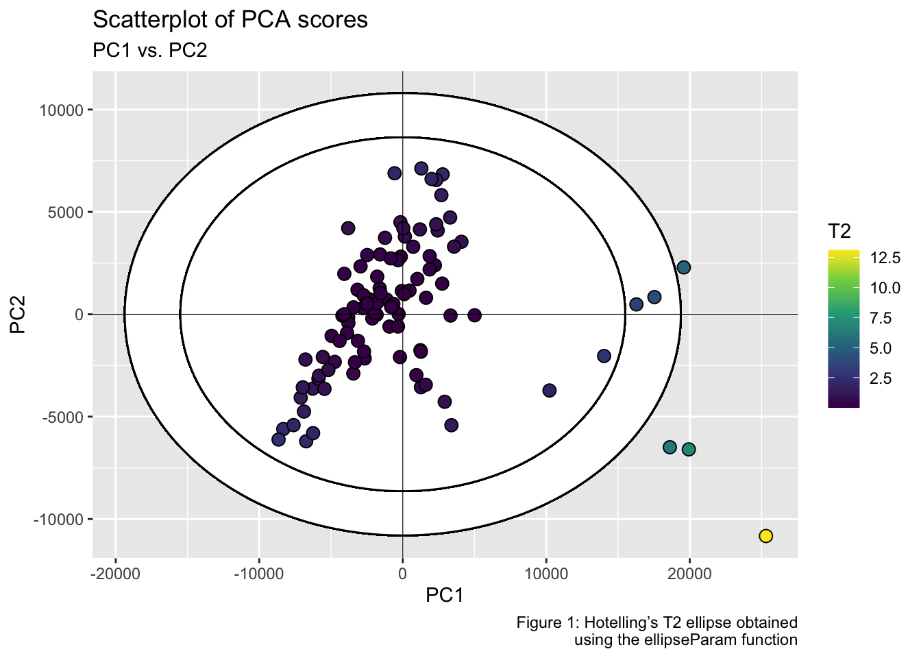
Or in the PC1-PC3 subspace at the confidence intervals set at 99, 95 and 90%.
ggplot() +
  geom_polygon(data = coord_2PCs_99, aes(x, y), color = "black", fill = "white") +
  geom_path(data = coord_2PCs_95, aes(x, y), color = "darkred") +
  geom_path(data = coord_2PCs_90, aes(x, y), color = "darkblue") +
  geom_point(data = pca_scores, aes(x = Dim.1, y = Dim.3, fill = T2), shape = 21, size = 3, color = "black") +
  scale_fill_viridis_c(option = "viridis") +
  geom_hline(yintercept = 0, linetype = "solid", color = "black", linewidth = .2) +
  geom_vline(xintercept = 0, linetype = "solid", color = "black", linewidth = .2) +
  labs(title = "Scatterplot of PCA scores", subtitle = "PC1 vs. PC3", x = "PC1", y = "PC3", fill = "T2", caption = "Figure 2: Hotelling’s T2 ellipse obtained\n using the ellipseCoord function") +
  theme_grey()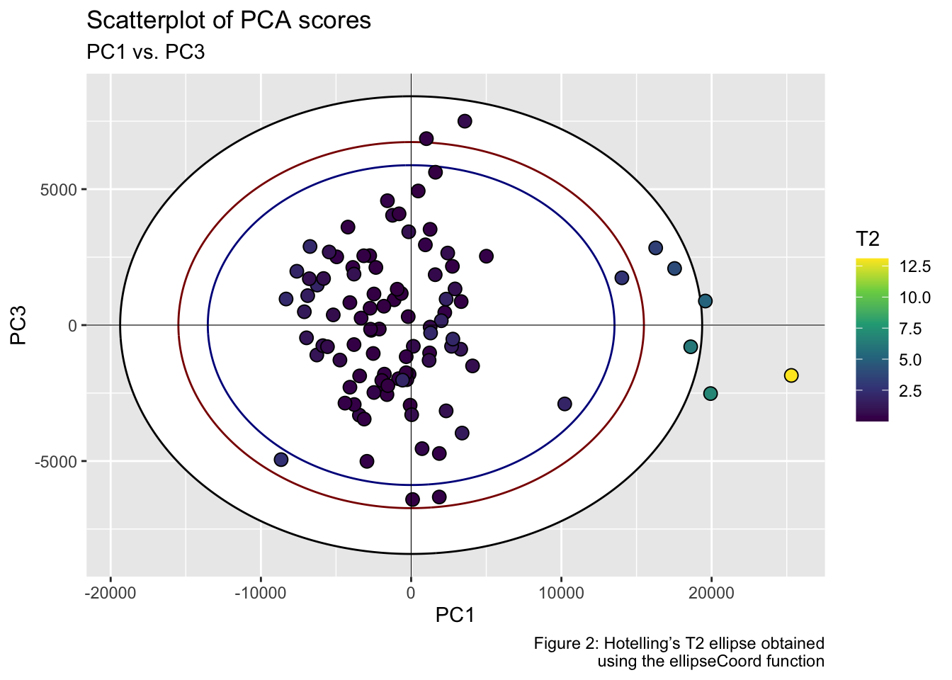
Note 1: Hotelling’s T-squared Ellipsoid - Visualizing Multivariate Data in 3D Space.
The ellipseCoord function has an optional parameter
pcz, which is set to NULL by default. When
specified, this parameter enables the computation of coordinates for
Hotelling’s T-squared ellipsoid in three-dimensional space. In the
example below, the 1st, 2nd, and 3rd components are mapped to the
x, y, and z-axis, respectively. The resulting
ellipsoid serves as a three-dimensional confidence region, encompassing
a specified proportion of the data points based on the chosen confidence
level.
df_ellipsoid <- ellipseCoord(pca_scores, pcx = 1, pcy = 2, pcz = 3, pts = 50)str(df_ellipsoid)
#> tibble [2,500 × 3] (S3: tbl_df/tbl/data.frame)
#> $ x: num [1:2500] -2.32e-13 -2.32e-13 -2.32e-13 -2.32e-13 -2.32e-13 ...
#> $ y: num [1:2500] 6.93e-13 6.93e-13 6.93e-13 6.93e-13 6.93e-13 ...
#> $ z: num [1:2500] 7745 7745 7745 7745 7745 ...T2 <- ellipseParam(pca_scores, k = 3)$Tsquare$valuecolor_palette <- viridisLite::viridis(nrow(pca_scores))
scaled_T2 <- scales::rescale(T2, to = c(1, nrow(pca_scores)))
point_colors <- color_palette[round(scaled_T2)]rgl::setupKnitr(autoprint = TRUE)
rgl::plot3d(
x = df_ellipsoid$x,
y = df_ellipsoid$y,
z = df_ellipsoid$z,
xlab = "PC1",
ylab = "PC2",
zlab = "PC3",
type = "l",
lwd = 0.5,
col = "lightgray",
alpha = 0.5)
rgl::points3d(
x = pca_scores$Dim.1,
y = pca_scores$Dim.2,
z = pca_scores$Dim.3,
col = point_colors,
size = 5,
add = TRUE)
rgl::bgplot3d({
par(mar = c(0,0,0,0))
plot.new()
color_legend <- as.raster(matrix(rev(color_palette), ncol = 1))
rasterImage(color_legend, 0.85, 0.1, 0.9, 0.9)
text(
x = 0.92,
y = seq(0.1, 0.9, length.out = 5),
labels = round(seq(min(T2), max(T2), length.out = 5), 2),
cex = 0.7)
text(x = 0.92, y = 0.95, labels = "T2", cex = 0.8)})
rgl::view3d(theta = 30, phi = 25, zoom = .8)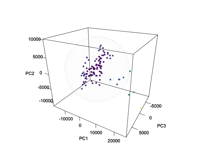
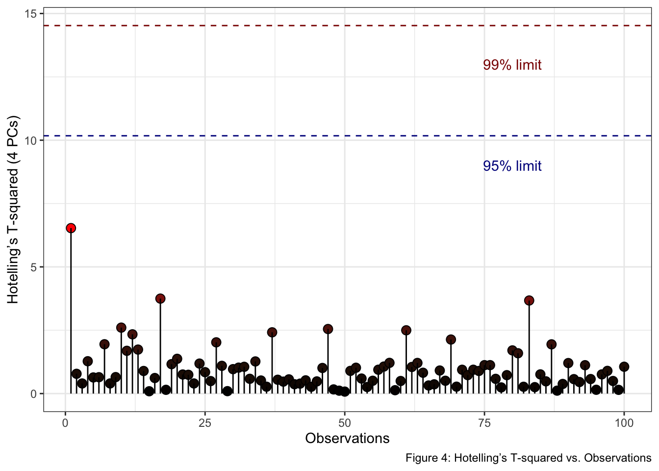
Note 2: Analysis of Hotelling’s T-squared Using Multiple Components.
When dealing with more than two principal components, visualizing Hotelling’s T-squared becomes challenging in traditional 2D or 3D plots. A more effective approach for analyzing and interpreting this multivariate statistic involves plotting Hotelling’s T-squared against Observations, where the confidence limits are plotted as a line. Thus, observations below the two lines are within the Hotelling’s T-squared limits.
In the provided example, we utilize the ellipseParam()
function with a cumulative variance threshold of 0.95
(threshold = 0.95). This setting ensures that the analysis
captures 95% of the total variance in the data.
df <- ellipseParam(pca_scores, threshold = 0.95)str(df)
#> List of 4
#> $ Tsquare : tibble [100 × 1] (S3: tbl_df/tbl/data.frame)
#> ..$ value: num [1:100] 6.53 0.78 0.399 1.276 0.636 ...
#> $ cutoff.99pct: num 14.5
#> $ cutoff.95pct: num 10.2
#> $ nb.comp : num 4tibble(
T2 = pluck(df, "Tsquare", "value"),
obs = 1:nrow(pca_scores)
) %>%
ggplot() +
geom_point(aes(x = obs, y = T2, fill = T2), shape = 21, size = 3, color = "black") +
geom_segment(aes(x = obs, y = T2, xend = obs, yend = 0), size = .5) +
scale_fill_gradient(low = "black", high = "red", guide = "none") +
geom_hline(yintercept = pluck(df, "cutoff.99pct"), linetype = "dashed", color = "darkred", linewidth = .5) +
geom_hline(yintercept = pluck(df, "cutoff.95pct"), linetype = "dashed", color = "darkblue", linewidth = .5) +
annotate("text", x = 80, y = 13, label = "99% limit", color = "darkred") +
annotate("text", x = 80, y = 9, label = "95% limit", color = "darkblue") +
labs(x = "Observations", y = "Hotelling’s T-squared (4 PCs)", fill = "T2 stats", caption = "Figure 4: Hotelling’s T-squared vs. Observations") +
theme_bw()
#> Warning: Using `size` aesthetic for lines was deprecated in ggplot2 3.4.0.
#> ℹ Please use `linewidth` instead.
#> This warning is displayed once every 8 hours.
#> Call `lifecycle::last_lifecycle_warnings()` to see where this warning was
#> generated.