

The goal of IRCcheck is to check the irrepresentable condition in both L1-regularized regression (Equation 2 in Zhao and Yu 2006) and Gaussian graphical models (Equation 8 in Ravikumar et al. 2008). At it crux, the IRC states that the important and unimportant variables cannot be correlated, at least not all that much (total irrelevant covariance below 1).
L1-regularization requires the IRC for consistent model selection, that is, with more data, the true model is recovered.
The IRC cannot be checked in real data. The primary use for this package is to explore the IRC in a true model that may be used in a simulation study. Alternatively, it is very informative to simply look at the IRC as a function of sparsity and the number of variables, including the regularization path and model selection.
You can install the development version from GitHub with:
# install.packages("devtools")
devtools::install_github("donaldRwilliams/IRCcheck")Here it is assumed that there is no covariance between the important (active) and unimportant variables.
library(IRCcheck)
# install from github
library(GGMnonreg)
library(GGMncv)
library(corrplot)
library(corpcor)
library(glmnet)
library(MASS)
library(psych)

# block diagonal
cors <- irc_met <- rbind(
  cbind(matrix(.7, 10,10), matrix(0, 10,10)),
  cbind(matrix(0, 10,10), matrix(0.7, 10,10))
)
diag(cors) <- 1


# visualize
# note: first 10 are 'active'
corrplot(cors)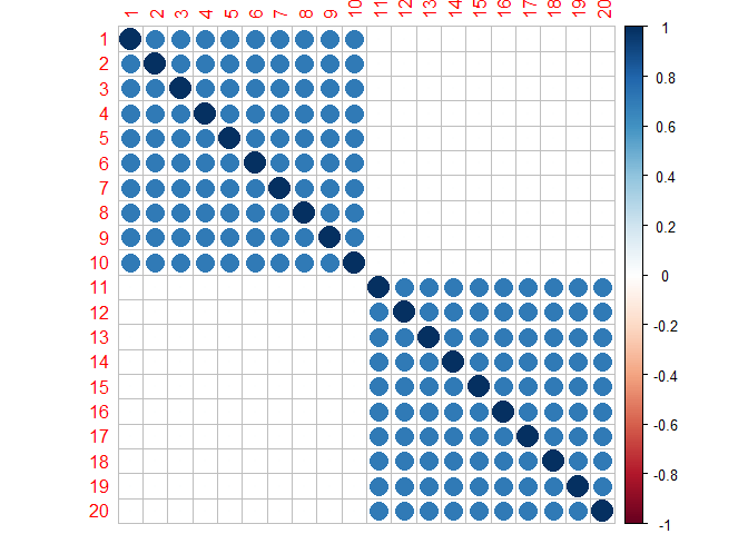
In this plot, variables 1 through 10 and 11 through 20 are correlated with each other. The latter are assumed to be “active” for predicting the response and the former are truly null associations. Notice there is no correlation between the sets.
Let’s inspect the regularization path
# beta
beta <- c(rep(1, 10), rep(0, 10))

set.seed(2)
X <- MASS::mvrnorm(n = 500, mu = rep(0, 20), Sigma = cors)

# SNR = 5
sigma <- sqrt(as.numeric(crossprod(beta, cors %*% beta) / 5))

set.seed(2)
# note: first 10 are 'active'
y <- X %*% c(rep(1, 10), rep(0, 10)) + rnorm(500, 0, sigma)

# fit model
fit <- glmnet(X, y)

# visualize
plot(fit, xvar = "lambda")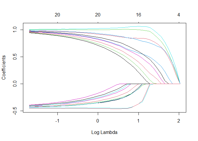
Here I generate a correlation matrix from a Wishart distribution.
# random correlation matrix
set.seed(2)
cors <- cov2cor(
  solve(
    rWishart(1, 20 , diag(20))[,,1]
  ))

# visualize
corrplot(cors)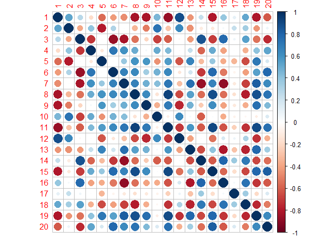
Now there are correlations between the sets, which, in my experience, is the more realistic situation (albeit these are very strong correlations).
Here is how to check the IRC in regression with IRCcheck
# SNR = 5
sigma <- sqrt(as.numeric(crossprod(beta, cors %*% beta) / 5))

set.seed(2)
X <- MASS::mvrnorm(n = 500, mu = rep(0, 20), Sigma = cors)

# if negative it is not met
1 - irc_regression(X, 1:10)
#> [1] -0.9509886
Let’s inspect the regularization path
set.seed(2)
y <- X %*% c(rep(1, 10), rep(0, 10)) + rnorm(500, 0, sigma)

# fit model
fit <- glmnet(X, y)

# visualize
plot(fit, xvar = "lambda")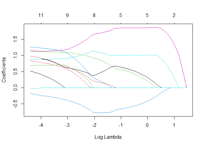
Quite the difference (e.g., all true coefficients are positive). Note that the goal is then to select lambda, which will be quite the difficult task when the IRC is not satisfied.
For GGMs, I find it easier to work with a partial correlation matrix and then randomly take subsets. The following looks at partial correlations estimated from items assessing personality.
# partials from big 5 data
pcors <- corpcor::cor2pcor(cor(na.omit(psych::bfi[,1:25])))

# collect
irc <- NA

for(i in 1:10){

   # randomly select 20
  id <- sample(1:25, size = 20, replace = F)

  # submatrix
  pcor_sub <- pcors[id, id]

  # true network
  true_net <- ifelse(abs(pcor_sub) < 0.05, 0, pcor_sub)

  irc[i] <- irc_ggm(true_net)
}

hist(1- irc, breaks = 100,
     xlab = "1 - infinity norm",
     main = "", xlim  = c(min(1 - irc), 1))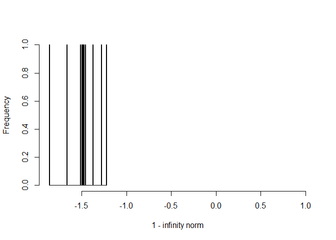
# failed
mean(1 - irc < 0)
#> [1] 1
Note that negative fails, as the irrelevant covariance exceeded 1. In fact, the IRC was not satisfied in any of the checks (10 iterations).
The IRC will fail less often with fewer variables. Also, if
0.05 is changed to a larger value this will result in more
sparsity. As a result, the IRC will be satisfied more often.
It might be tempting to think that violating IRC, like many other assumptions, will have some effect but perhaps not all that much. In my experience, the importance of the IRC cannot be understated: it has a HUGE impact on false positives. The following is a somewhat “ugly” example.
Let’s hold all constant (p and effect size) but sparsity and examine
the infinity norm (must be less than 1). Below, gen_net
generates a true network, or GGM, with partial correlations in a certain
range (lb and ub).
# 5 % connections (95 % sparsity)
eprob_05 <- IRCcheck::gen_net(
  p = 10,
  edge_prob = 0.05,
  lb = 0.05,
  ub = 0.25
)

# 25 % connections (75 % sparsity)
eprob_25 <- IRCcheck::gen_net(
  p = 10,
  edge_prob = 0.25,
  lb = 0.05,
  ub = 0.25
)

# most networks in the social-behavioral sciences are **not** sparse
# 50 % connections (50 % sparsity)
eprob_50 <- IRCcheck::gen_net(
  p = 10,
  edge_prob = 0.50,
  lb = 0.05,
  ub = 0.25
)

# 75 % connections (25 % sparsity)
eprob_75 <- IRCcheck::gen_net(
  p = 10,
  edge_prob = 0.75,
  lb = 0.05,
  ub = 0.25
)

# compute infinity norms
ircs <-
  sapply(list(eprob_05,
              eprob_25,
              eprob_50,
              eprob_75), function(x) {
    IRCcheck::irc_ggm(x$pcors)
  })

# plot
plot(
  c(0.05, 0.25, 0.50, 0.75),
  1 - ircs,
  cex = 2,
  ylab = "1 - Infinity Norm",
  xlab = "Edge Probability (Connectivity)"
)
abline(h = 0)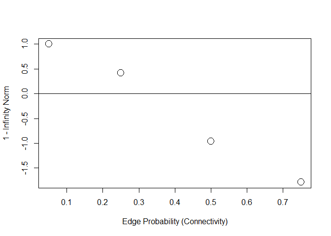
Because I subtracted 1, negative values fail to meet the IRC. As the graph becomes less sparse (higher edge probability) the infinity norm becomes larger, i.e., the covariance between the unimportant and important increases, which should translate into more false positives.
Now let’s check specificity (1 - the false positive) in simulated data. At each step, the IRC is increasingly violated.
set.seed(1)
# data
Y <- MASS::mvrnorm(n = 5000,
                   rep(0, 10),
                   Sigma = eprob_05$cors,
                   empirical = FALSE)

# non regularized, for comparison
fit <- GGMnonreg::ggm_inference(Y, boot = FALSE)

# specificity
IRCcheck:::compare(True = eprob_05$adj,
                   Estimate = fit$adj)[1,]
#>       measure     score
#> 1 Specificity 0.9767442

# lasso
fit <- GGMncv::ggmncv(cor(Y), n = 5000,
                      penalty = "lasso",
                      progress = FALSE)

# specificity
IRCcheck:::compare(True = eprob_05$adj,
                   Estimate = fit$adj)[1,]
#>       measure     score
#> 1 Specificity 0.9767442
Notice that both methods work well.
set.seed(1)
# data
Y <- MASS::mvrnorm(n = 5000,
                   rep(0, 10),
                   Sigma = eprob_25$cors,
                   empirical = FALSE)

# non regularized, for comparison
fit <- GGMnonreg::ggm_inference(Y, boot = FALSE)

# specificity
IRCcheck:::compare(True = eprob_25$adj,
                   Estimate = fit$adj)[1,]
#>       measure score
#> 1 Specificity     1

# lasso
fit <- GGMncv::ggmncv(cor(Y),
              n = 5000,
              penalty = "lasso",
              progress = FALSE)

# specificity
IRCcheck:::compare(True = eprob_25$adj,
        Estimate = fit$adj)[1,]
#>       measure     score
#> 1 Specificity 0.8235294Now we are getting to a level of sparsity that is common in, say, the social-behavioral sciences.
set.seed(1)
# data
Y <- MASS::mvrnorm(n = 5000,
                   rep(0, 10),
                   Sigma = eprob_50$cors,
                   empirical = FALSE)

# non regularized, for comparison
fit <- GGMnonreg::ggm_inference(Y, boot = FALSE)

# specificity
IRCcheck:::compare(True = eprob_50$adj,
                   Estimate = fit$adj)[1,]
#>       measure     score
#> 1 Specificity 0.9130435

# lasso
fit <- GGMncv::ggmncv(cor(Y),
              n = 5000,
              penalty = "lasso",
              progress = FALSE)

# specificity
IRCcheck:::compare(True = eprob_50$adj,
        Estimate = fit$adj)[1,]
#>       measure     score
#> 1 Specificity 0.3913043An even denser graph, which is not uncommon.
set.seed(1)
# data
Y <- MASS::mvrnorm(n = 5000,
                   rep(0, 10),
                   Sigma = eprob_75$cors,
                   empirical = FALSE)

# non regularized, for comparison
fit <- GGMnonreg::ggm_inference(Y, boot = FALSE)

# specificity
IRCcheck:::compare(True = eprob_75$adj,
                   Estimate = fit$adj)[1,]
#>       measure score
#> 1 Specificity     1

# lasso
fit <- GGMncv::ggmncv(cor(Y),
              n = 5000,
              penalty = "lasso",
              progress = FALSE)

# specificity
IRCcheck:::compare(True = eprob_75$adj,
        Estimate = fit$adj)[1,]
#>       measure score
#> 1 Specificity     0

# false positive rate
1 - IRCcheck:::compare(True = eprob_75$adj,
            Estimate = fit$adj)[1,2]
#> [1] 1
At each step along the way, the false positive rate for (g)lasso increased to be shockingly high. On the other hand, the non-regularized method based on good old p-values had no issue.
Together, this simple example demonstrated that the false positive rate is a function of the IRC.
Ravikumar, Pradeep, Garvesh Raskutti, Martin J Wainwright, and Bin Yu. 2008. “Model Selection in Gaussian Graphical Models: High-Dimensional Consistency of L1-Regularized Mle.” In NIPS, 1329–36.
Zhao, Peng, and Bin Yu. 2006. “On Model Selection Consistency of Lasso.” The Journal of Machine Learning Research 7: 2541–63. https://doi.org/10.1109/TIT.2006.883611.