SSIMmap

The goal of SSIMmap is to extend the classical Structural Similarity Index Measure (SSIM) — originally developed for image quality assessment — to maps. The package provides a unified framework for quantifying spatial similarity between two maps of the same area, for both irregular polygon (lattice) data and raster images.

For polygon maps, the geographical SSIM method incorporates geographically weighted summary statistics with an adaptive k-nearest-neighbor Gaussian kernel. For raster images, SSIM is computed using a moving window. In addition to point estimates, SSIMmap also supports permutation tests for both global and local significance, with optional Benjamini–Hochberg FDR correction.

Key features

• ssim_bandwidth() — bias–variance trade-off plots to help choose an appropriate bandwidth (number of neighbors k) for polygon maps.
• ssim_polygon() — global and local SSIM (and components SIM, SIV, SIP) for polygon maps, with permutation testing and FDR correction.
• ssim_raster() — global and local SSIM for raster images, with permutation testing and per-cell p-/q-values.
• Multiple value transforms ("normal_score", "percentile", "minmax", "none") for comparing variables on different scales.
• Built-in example data: Toronto 2021 Aggregate Dissemination Area deprivation indices (Toronto_SSIM) and British Columbia Fire Weather Index rasters (fwi_0816_bc, fwi_0818_bc, fwi_1111_bc, plus the legacy fwi_1101_bc).

Installation

Install the released version from CRAN:

install.packages("SSIMmap")

The current defaults and two-sided raster examples below require SSIMmap 0.4.2 or later.

The development version is available from GitHub:

# install.packages("remotes")
remotes::install_github("Hailyee-Ha/SSIMmap", build_vignettes = TRUE)

Quick example

library(SSIMmap)
library(sf)
library(terra)
library(ggplot2)
library(patchwork)
library(tidyterra)

Example 1 — Polygon maps: comparing two deprivation indices in Toronto

The package ships with Toronto_SSIM, an sf object containing 279 Aggregate Dissemination Areas (ADAs) for Toronto from the 2021 Census geography. It includes a Canadian Index of Multiple Deprivation residential instability score (CIMD) and the social dimension of the Pampalon index (PP), plus a derived commuting measure (Commute). Its numeric data are unchanged from version 0.4.0. Commute is the unweighted mean of all stored DA percentages for all intersecting DAs, including boundary-only intersections and stored zeros. The nine zero-population DAs have stored zero percentages, which are included in the means. For positive-population DAs, the percentage is 100 times the Census count for commuting to a different CSD and CD within the province or territory of residence (characteristic 2601), divided by total DA Census population (characteristic 1), rounded half-up to two decimals. It is not a household or worker share, a pooled ADA population rate, or the share of all commuting outside the CSD. Sixteen source numerator cells are officially suppressed but stored as zero in the preserved source; their values cannot be independently verified from the public release. See the installed extdata/Toronto_SSIM_provenance.txt note.

data("Toronto_SSIM")

p_cimd <- ggplot(Toronto_SSIM) +
  geom_sf(aes(fill = CIMD), color = NA) +
  scale_fill_viridis_c(option = "magma") +
  labs(title = "CIMD") + theme_void()

p_pp <- ggplot(Toronto_SSIM) +
  geom_sf(aes(fill = PP), color = NA) +
  scale_fill_viridis_c(option = "magma") +
  labs(title = "Pampalon") + theme_void()

p_cimd + p_pp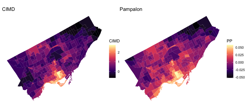

Step 1: Choose a bandwidth

ssim_bandwidth() provides a bias–variance trade-off curve for selecting k, the number of nearest neighbors used in the adaptive kernel.

S <- ssim_bandwidth(
  shape         = Toronto_SSIM,
  map1          = "CIMD",
  map2          = "PP",
  max_bandwidth = 200,
  transform     = "percentile",
  option        = "midpoint"
)
S$bandwidth
#> [1] 87
S$plot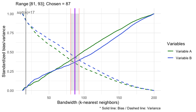

Step 2: Compute global SSIM with a permutation test

S_global <- ssim_polygon(
  shape     = Toronto_SSIM,
  map1      = "CIMD",
  map2      = "PP",
  global    = TRUE,
  bandwidth = S$bandwidth,
  transform = "percentile",
  do_test   = TRUE, R = 1000, fdr = TRUE, alpha = 0.05,
  seed      = 1
)
S_global$p_global

Step 3: Compute descriptive local SSIM and visualize it

S_local <- ssim_polygon(
  shape     = Toronto_SSIM,
  map1      = "CIMD",
  map2      = "PP",
  global    = FALSE,
  bandwidth = S$bandwidth,
  transform = "percentile",
  do_test   = FALSE
)

ggplot(S_local) +
  geom_sf(aes(fill = SSIM), color = NA) +
  scale_fill_distiller(palette = "PRGn", limits = c(-1, 1)) +
  labs(title = "Local SSIM: CIMD vs. Pampalon") +
  theme_void()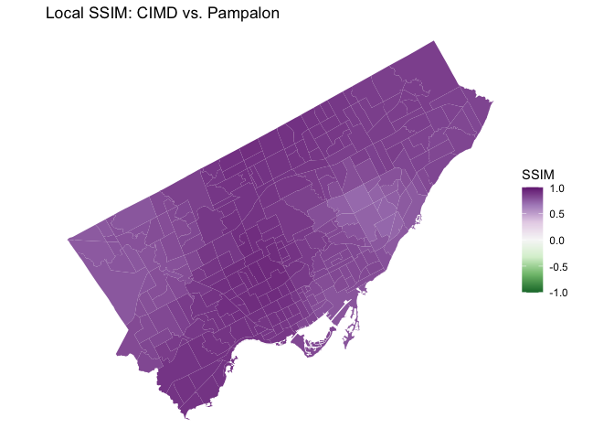

The S_local object is an ordinary sf data frame, so you can also map its components (SIM, SIV, SIP). From version 0.4.3, repeat the local call with do_test = TRUE, R = 1000, and a fixed seed to obtain two-sided local tests for all four statistics. Columns use _p, _q, and _sig suffixes, for example SIM_p, SIM_q, and SIM_sig. BH correction is applied across polygons separately for each statistic. Both polygon and raster significance use q <= alpha, or p <= alpha without FDR adjustment. The existing p_value, q_value, and sig columns remain aliases for the SSIM results. With fdr = FALSE, polygon _q columns equal their unadjusted p-values.

Example 2 — Raster maps: comparing daily Fire Weather Index in British Columbia

The manuscript examples use three daily Canadian Fire Weather Index (FWI) maps for British Columbia at 2 km resolution: 16 and 18 August 2023 and 11 November 2023. Version 0.4.1 adds the actual November 11 observation as fwi_1111_bc. The earlier fwi_1101_bc remains the unchanged November 1 observation for compatibility. These are distinct data, not alternative names for one raster.

The examples explicitly use transform = "none" to compare original FWI values. From version 0.4.2, "none" is the default in ssim_raster(), ssim_polygon(), and ssim_bandwidth(). Use transform = "percentile" explicitly for the Toronto comparisons shown above.

From version 0.4.2, both global and local raster permutation tests are two-sided, using distance from the permutation mean, as in the polygon tests. Raster map A remains fixed while map B is shuffled over common valid cells. Observed SSIM components are unchanged for an explicitly selected transformation; p-values, BH-adjusted q-values, and significance flags can change. Local tests replay the same draws in two passes to avoid storing all null rasters.

data("fwi_0816_bc"); fwi_0816_bc <- terra::unwrap(fwi_0816_bc)
data("fwi_0818_bc"); fwi_0818_bc <- terra::unwrap(fwi_0818_bc)
data("fwi_1111_bc"); fwi_1111_bc <- terra::unwrap(fwi_1111_bc)

par(mfrow = c(1, 3))
plot(fwi_0816_bc, main = "FWI – 16 Aug 2023", range = c(0, 110))
plot(fwi_0818_bc, main = "FWI – 18 Aug 2023", range = c(0, 110))
plot(fwi_1111_bc, main = "FWI – 11 Nov 2023", range = c(0, 110))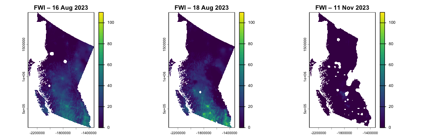

All three input-map panels use the same 0–110 FWI color scale.

Global SSIM

A quick global comparison (no permutation test, fast):

ssim_raster(fwi_0816_bc, fwi_0818_bc, w = 1, transform = "none") # summer vs summer
#> $summary
#>   metric      mean        min       max         sd
#> 1   SSIM 0.7686929 -0.1976864 0.9999991 0.29695831
#> 2    SIM 0.7888708  0.0034073 1.0000000 0.29035795
#> 3    SIV 0.9603730  0.1852894 1.0000000 0.08892729
#> 4    SIP 0.9915390 -0.2499358 1.0000000 0.02908319
#> 
#> $settings
#> $settings$global
#> [1] TRUE
#> 
#> $settings$w
#> [1] 1
#> 
#> $settings$transform
#> [1] "none"
#> 
#> $settings$do_test
#> [1] FALSE
#> 
#> $settings$local_test
#> [1] FALSE
ssim_raster(fwi_0816_bc, fwi_1111_bc, w = 1, transform = "none") # summer vs fall
#> $summary
#>   metric      mean           min max         sd
#> 1   SSIM 0.2259786 -0.2139426534   1 0.33614608
#> 2    SIM 0.2339652  0.0001376689   1 0.33838033
#> 3    SIV 0.7107652  0.0308876725   1 0.28760524
#> 4    SIP 0.9940730 -0.2700576644   1 0.03425971
#> 
#> $settings
#> $settings$global
#> [1] TRUE
#> 
#> $settings$w
#> [1] 1
#> 
#> $settings$transform
#> [1] "none"
#> 
#> $settings$do_test
#> [1] FALSE
#> 
#> $settings$local_test
#> [1] FALSE

As expected, the summer–summer comparison shows much higher similarity than the summer–fall comparison.

Local SSIM and components

For per-cell SSIM surfaces, set global = FALSE. Below we use tidyterra to faceted-plot the four SSIM components:

p1_l <- ssim_raster(
  fwi_0816_bc, fwi_0818_bc,
  global = FALSE, w = 1, transform = "none"
)

ggplot() +
  geom_spatraster(data = p1_l[[c("SSIM", "SIM", "SIV", "SIP")]]) +
  facet_wrap(~lyr, ncol = 2) +
  scale_fill_viridis_c(limits = c(-1, 1), na.value = "transparent") +
  theme_minimal()

Setting do_test = TRUE and local_test = TRUE additionally returns per-cell permutation p-values (SSIM_p, SIM_p, SIV_p, SIP_p) and FDR-adjusted q-values (SSIM_q, …).

Reproduce the manuscript

The installed package includes the analytical inputs, fixed seeds, scripts and reference results for both tables and Figures 3–7. No external download or computer-specific path is required. Run in a new writable output directory:

source(system.file("reproduction", "reproduce_manuscript.R",
                   package = "SSIMmap"))
reproduce_manuscript("ssim-observed", full = FALSE)
reproduce_manuscript("ssim-full", full = TRUE)

The first call verifies observed values and bandwidths. The second also runs all 1,000-permutation tests, including the local significance maps. It is a long-running analysis, rather than a package example run during installation. See the installed reproduction/README.txt for settings, separate-job execution, verification tolerances and the scope of historical Toronto source reconstruction. Rendering instructions are included under system.file("figures", package = "SSIMmap").

The November 11 FWI was verified against the historical coverage provided by Natural Resources Canada, Canadian Forest Service, CWFIS. The original grid, missing cells and all values match the official coverage. Exact retrieval parameters and attribution are in extdata/fwi_1111_bc_provenance.txt.

Learn more

A more detailed walkthrough — including bandwidth selection, side-by-side patchwork plots, and tidyterra styling for publication-ready figures — is available in the package vignette:

vignette("Introduction_to_SSIMmap", package = "SSIMmap")

Or, after installing from GitHub with build_vignettes = TRUE, browse all vignettes:

browseVignettes("SSIMmap")

Citation

If you use SSIMmap in your research, please cite both the package and the original SSIM paper:

citation("SSIMmap")

• Wang, Z., Bovik, A.C., Sheikh, H.R. and Simoncelli, E.P. (2004). Image quality assessment: from error visibility to structural similarity. IEEE Transactions on Image Processing, 13(4), 600–612. https://doi.org/10.1109/TIP.2003.819861
• Brunsdon, C., Fotheringham, A.S. and Charlton, M. (2002). Geographically weighted summary statistics — a framework for localised exploratory data analysis. Computers, Environment and Urban Systems, 26(6), 501–524. https://doi.org/10.1016/S0198-9715(01)00009-6

Contributing & bug reports

Bug reports, feature requests, and pull requests are very welcome — please open an issue on GitHub.

License

MIT © Hui Jeong (Hailyee) Ha and Jed Long.

The November 11 FWI data contain information licensed under the Open Government Licence – Canada. Source: Canadian Forest Service. 2022. Canadian Wildland Fire Information System (CWFIS), Natural Resources Canada, Canadian Forest Service, Northern Forestry Centre, Edmonton, Alberta. See the installed provenance note for source metadata.