You can install autoReg package on github.
#install.packages("devtools")
devtools::install_github("cardiomoon/autoReg")To load the package, use library() function.
library(autoReg)You can make a table summarizing baseline characteristics easily.
library(moonBook) # For use of example data acs
gaze(sex~.,data=acs)
————————————————————————————————————————————————————————————————————————
  Dependent:sex        levels           Female          Male        p
       (N)                             (N=287)        (N=570)
————————————————————————————————————————————————————————————————————————
age               Mean ± SD             68.7 ± 10.7   60.6 ± 11.2  <.001
cardiogenicShock  No                    275 (95.8%)     530 (93%)   .136
                  Yes                     12 (4.2%)       40 (7%)
entry             Femoral               119 (41.5%)   193 (33.9%)   .035
                  Radial                168 (58.5%)   377 (66.1%)
Dx                NSTEMI                 50 (17.4%)   103 (18.1%)   .012
                  STEMI                  84 (29.3%)   220 (38.6%)
                  Unstable Angina       153 (53.3%)   247 (43.3%)
EF                Mean ± SD             56.3 ± 10.1    55.6 ± 9.4   .387
height            Mean ± SD             153.8 ± 6.2   167.9 ± 6.1  <.001
weight            Mean ± SD              57.2 ± 9.3   68.7 ± 10.3  <.001
BMI               Mean ± SD              24.2 ± 3.6    24.3 ± 3.2   .611
obesity           No                    194 (67.6%)   373 (65.4%)   .580
                  Yes                    93 (32.4%)   197 (34.6%)
TC                Mean ± SD            188.9 ± 51.1  183.3 ± 45.9   .124
LDLC              Mean ± SD            117.8 ± 41.2  116.0 ± 41.1   .561
HDLC              Mean ± SD             39.0 ± 11.5   37.8 ± 10.9   .145
TG                Mean ± SD            119.9 ± 76.2  127.9 ± 97.3   .195
DM                No                    173 (60.3%)   380 (66.7%)   .077
                  Yes                   114 (39.7%)   190 (33.3%)
HBP               No                     83 (28.9%)   273 (47.9%)  <.001
                  Yes                   204 (71.1%)   297 (52.1%)
smoking           Ex-smoker              49 (17.1%)   155 (27.2%)  <.001
                  Never                 209 (72.8%)   123 (21.6%)
                  Smoker                 29 (10.1%)   292 (51.2%)
————————————————————————————————————————————————————————————————————————You can make a publication-ready table easily using myft(). It makes a flextable object which can use in either HTML and PDF format.
library(dplyr) # for use of `%>%`

Attaching package: 'dplyr'
The following objects are masked from 'package:stats':

    filter, lag
The following objects are masked from 'package:base':

    intersect, setdiff, setequal, union
ft=gaze(sex~.,data=acs) %>% myft()
ft
You can also make a powerpoint file using rrtable::table2pptx() function.
library(rrtable)

table2pptx(ft)
Exported table as Report.pptxYou can make a microsoft word file using rrtable::table2docx() function.
table2docx(ft)Exported table as Report.docxYou can get a table summarizing baseline characteristics with two or more grouping variables.
gaze(sex+Dx~.,data=acs) %>% myft()
You can also use three or more grouping variables.The resultant table will be too long to review, but you can try.
gaze(sex+DM+HBP~age,data=acs) %>% myft()
You can make a table summarizing results of regression analysis. For example, let us perform a logistic regression with the colon cancer data.
library(survival)   # For use of data colon
data(cancer)

fit=glm(status~rx+sex+age+obstruct+perfor+nodes,data=colon,family="binomial")
summary(fit)

Call:
glm(formula = status ~ rx + sex + age + obstruct + perfor + nodes,
    family = "binomial", data = colon)

Deviance Residuals:
    Min       1Q   Median       3Q      Max
-2.4950  -1.0594  -0.7885   1.1619   1.6424

Coefficients:
             Estimate Std. Error z value Pr(>|z|)
(Intercept) -0.645417   0.285558  -2.260   0.0238 *
rxLev       -0.067422   0.118907  -0.567   0.5707
rxLev+5FU   -0.627480   0.121684  -5.157 2.51e-07 ***
sex         -0.053541   0.098975  -0.541   0.5885
age          0.002307   0.004234   0.545   0.5859
obstruct     0.283703   0.125194   2.266   0.0234 *
perfor       0.319281   0.292034   1.093   0.2743
nodes        0.190563   0.018255  10.439  < 2e-16 ***
---
Signif. codes:  0 '***' 0.001 '**' 0.01 '*' 0.05 '.' 0.1 ' ' 1

(Dispersion parameter for binomial family taken to be 1)

    Null deviance: 2525.4  on 1821  degrees of freedom
Residual deviance: 2342.4  on 1814  degrees of freedom
  (36 observations deleted due to missingness)
AIC: 2358.4

Number of Fisher Scoring iterations: 4
You can make table with above result.
autoReg(fit)
——————————————————————————————————————————————————————————————————————————————————
 Dependent: status              0 (N=925)    1 (N=897)      OR (multivariable)
——————————————————————————————————————————————————————————————————————————————————
rx                 Obs          282 (30.5%)  342 (38.1%)
                   Lev          285 (30.8%)    323 (36%)  0.93 (0.74-1.18, p=.571)
                   Lev+5FU      358 (38.7%)  232 (25.9%)  0.53 (0.42-0.68, p<.001)
sex                Mean ± SD      0.5 ± 0.5    0.5 ± 0.5  0.95 (0.78-1.15, p=.589)
age                Mean ± SD    60.1 ± 11.5  59.5 ± 12.3  1.00 (0.99-1.01, p=.586)
obstruct           Mean ± SD      0.2 ± 0.4    0.2 ± 0.4  1.33 (1.04-1.70, p=.023)
perfor             Mean ± SD      0.0 ± 0.2    0.0 ± 0.2  1.38 (0.78-2.47, p=.274)
nodes              Mean ± SD      2.7 ± 2.4    4.6 ± 4.2  1.21 (1.17-1.26, p<.001)
——————————————————————————————————————————————————————————————————————————————————
Or you can make a publication-ready table.
autoReg(fit) %>% myft()
If you want make a table with more explanation, you can make categorical variables with numeric variables. For example, the explanatory variables obstruct(obstruction of colon by tumor) and perfor(perforation of colon) is coded as 0 or 1, but it is “No” or “Yes” actually. Also the dependent variable status is coded as 0 or 1, it is “Alive” or “Died”.
colon$status.factor=factor(colon$status,labels=c("Alive","Died"))
colon$obstruct.factor=factor(colon$obstruct,labels=c("No","Yes"))
colon$perfor.factor=factor(colon$perfor,labels=c("No","Yes"))
colon$sex.factor=factor(colon$sex,labels=c("Female","Male"))

fit=glm(status.factor~rx+sex.factor+age+obstruct.factor+perfor.factor+nodes,data=colon,family="binomial")
result=autoReg(fit)
result %>% myft()
You can add labels to the names of variables with setLabel() function.
colon$status.factor=setLabel(colon$status.factor,"Mortality")
colon$rx=setLabel(colon$rx,"Treatment")
colon$age=setLabel(colon$age,"Age(Years)")
colon$sex.factor=setLabel(colon$sex.factor,"Sex")
colon$obstruct.factor=setLabel(colon$obstruct.factor,"Obstruction")
colon$perfor.factor=setLabel(colon$perfor.factor,"Perforation")
colon$nodes=setLabel(colon$nodes,"Positive nodes")

fit=glm(status.factor~rx+sex.factor+age+obstruct.factor+perfor.factor+nodes,data=colon,family="binomial")
result=autoReg(fit)
result %>% myft()
If you do not want to show the reference values in table, you can shorten the table.
shorten(result) %>% myft()
You can add the results of univariate analyses to the table. At this time, the autoReg() function automatically select explanatory variables below the threshold(default value 0.2) and perform multivariate analysis. In this table, the p values of explanatory variables sex.factor and age is above the default threshold(0.2), they are excluded in multivariate model.
autoReg(fit, uni=TRUE) %>% myft()
If you want to include all explanatory variables in the multivariate model, just set the threshold 1.
autoReg(fit, uni=TRUE,threshold=1) %>% myft()
You can perform stepwise backward elimination to select variables and make a final model. Just set final=TRUE.
autoReg(fit, uni=TRUE,threshold=1, final=TRUE) %>% myft()
When the argument imputed=TRUE, autoReg() function make a multiple imputed model using mice::mice() function. By default, 20 imputations performed. If you want, you can change the number of imputations with m argument.
autoReg(fit, imputed=TRUE) %>% myft()
You can draw the plot summarizing the model with modelPlot()
x=modelPlot(fit)
x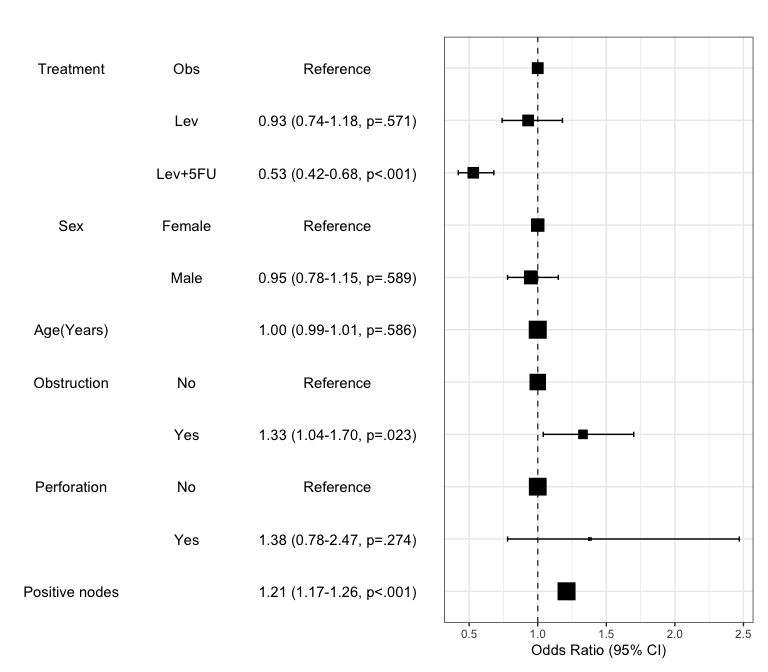
You can make powerpoint file with this plot using rrtable::plot2pptx().
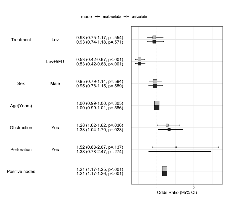
plot2pptx(print(x))Exported plot as Report.pptxYou can summarize models in a plot. If you want to summarize univariate and multivariate model in a plot, just set the uni=TRUE and adjust the threshold. You can decide whether or not show the reference by show.ref argument.
modelPlot(fit,uni=TRUE,threshold=1,show.ref=FALSE)