![]()
![]()
Density ratio estimation is described as follows:
for given two data samples x1 and x2 from
unknown distributions p(x) and q(x)
respectively, estimate w(x) = p(x) / q(x), where
x1 and x2 are d-dimensional real numbers.
The estimated density ratio function w(x) can be used in
many applications such as anomaly detection [Hido et
al. 2011], change-point detection [Liu et al. 2013],
and covariate shift adaptation [Sugiyama et al. 2007].
Other useful applications about density ratio estimation were summarized
by [Sugiyama et al. 2012].
The package densratio provides a function
densratio() that returns an object with a method to
estimate density ratio as compute_density_ratio().
For example,
set.seed(3)
x1 <- rnorm(200, mean = 1, sd = 1/8)
x2 <- rnorm(200, mean = 1, sd = 1/2)

library(densratio)
densratio_obj <- densratio(x1, x2)
The densratio object has a function
compute_density_ratio() that can compute the estimated
density ratio w_hat(x) for any d-dimensional input
x (now d=1).
new_x <- seq(0, 2, by = 0.03)
w_hat <- densratio_obj$compute_density_ratio(new_x)

plot(new_x, w_hat, pch=19)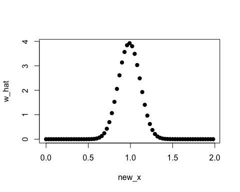
In this case, the true density ratio
w(x) = p(x)/q(x) = Norm(1, 1/8) / Norm(1, 1/2) is known. So
we can compare w(x) with the estimated density ratio
w-hat(x).
true_density_ratio <- function(x) dnorm(x, 1, 1/8) / dnorm(x, 1, 1/2)

plot(true_density_ratio, xlim=c(0, 2), lwd=2, col="red", xlab = "x", ylab = "Density Ratio")
plot(densratio_obj$compute_density_ratio, xlim=c(0, 2), lwd=2, col="green", add=TRUE)
legend("topright", legend=c(expression(w(x)), expression(hat(w)(x))), col=2:3, lty=1, lwd=2, pch=NA)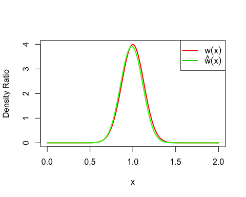
You can install the densratio package from CRAN.
install.packages("densratio")You can also install the package from GitHub.
install.packages("remotes") # if you have not installed "remotes" package
remotes::install_github("hoxo-m/densratio")
The source code for densratio package is available on GitHub at
The package provides densratio(). The function returns
an object that has a function to compute estimated density ratio.
For data samples x1 and x2,
set.seed(3)
x1 <- rnorm(200, mean = 1, sd = 1/8)
x2 <- rnorm(200, mean = 1, sd = 1/2)

library(densratio)
densratio_obj <- densratio(x1, x2)
In this case, densratio_obj$compute_density_ratio() can
compute estimated density ratio.
new_x <- seq(0, 2, by = 0.03)
w_hat <- densratio_obj$compute_density_ratio(new_x)

plot(new_x, w_hat, pch=19)
densratio() has method argument that you
can pass "uLSIF", "RuLSIF", or
"KLIEP".
The methods assume that density ratios are represented by linear model:
w(x) = theta_1 * K(x, c_1) + theta_2 * K(x, c_2) + ... + theta_b * K(x, c_b)where
K(x, c) = exp(-||x - c||^2 / (2 * sigma^2))is the Gaussian (RBF) kernel.
densratio() performs the following:
sigma by
cross-validation,theta (in other words,
find the optimal coefficients of the linear model), andsigma and theta are saved
into densratio object, and are used when to compute density
ratio in the call compute_density_ratio().densratio() outputs the result like as follows:
#>
#> Call:
#> densratio(x1 = x1, x2 = x2, method = "uLSIF")
#>
#> Kernel Information:
#>   Kernel type:  Gaussian
#>   Number of kernels:  100
#>   Bandwidth (sigma):  0.1
#>   Centers:  num [1:100, 1] 0.907 1.093 1.18 1.136 1.046 ...
#>
#> Kernel Weights:
#>   num [1:100] 0.067455 0.040045 0.000459 0.016849 0.067084 ...
#>
#> Regularization Parameter (lambda):  1
#>
#> Function to Estimate Density Ratio:
#> compute_density_ratio()kernel_num
argument. In default, kernel_num = 100.sigma = "auto", the algorithm automatically
select an optimal value by cross validation. If you set
sigma a number, that will be used. If you set
sigma a numeric vector, the algorithm select an optimal
value in them by cross validation.x1 underlying a numerator distribution p(x).
You can find the whole values in
result$kernel_info$centers.theta parameters in
the linear kernel model. You can find these values in
result$kernel_weights.compute_density_ratio().So far, the input data samples x1 and x2
were one dimensional. densratio() allows to input
multidimensional data samples as matrix, as long as their
dimensions are the same.
For example,
library(densratio)
library(mvtnorm)

set.seed(3)
x1 <- rmvnorm(300, mean = c(1, 1), sigma = diag(1/8, 2))
x2 <- rmvnorm(300, mean = c(1, 1), sigma = diag(1/2, 2))

densratio_obj_2d <- densratio(x1, x2)
densratio_obj_2d
#>
#> Call:
#> densratio(x1 = x1, x2 = x2, method = "uLSIF")
#>
#> Kernel Information:
#>   Kernel type:  Gaussian
#>   Number of kernels:  100
#>   Bandwidth (sigma):  0.316
#>   Centers:  num [1:100, 1:2] 1.257 0.758 1.122 1.3 1.386 ...
#>
#> Kernel Weights:
#>   num [1:100] 0.0756 0.0986 0.059 0.0797 0.0421 ...
#>
#> Regularization Parameter (lambda):  0.3162278
#>
#> Function to Estimate Density Ratio:
#>   compute_density_ratio()
In this case, as well, we can compare the true density ratio with the estimated density ratio.
true_density_ratio <- function(x) {
  dmvnorm(x, mean = c(1, 1), sigma = diag(1/8, 2)) /
    dmvnorm(x, mean = c(1, 1), sigma = diag(1/2, 2))
}

N <- 20
range <- seq(0, 2, length.out = N)
input <- expand.grid(range, range)
w_true <- matrix(true_density_ratio(input), nrow = N)
w_hat <- matrix(densratio_obj_2d$compute_density_ratio(input), nrow = N)

par(mfrow = c(1, 2))
contour(range, range, w_true, main = "True Density Ratio")
contour(range, range, w_hat, main = "Estimated Density Ratio")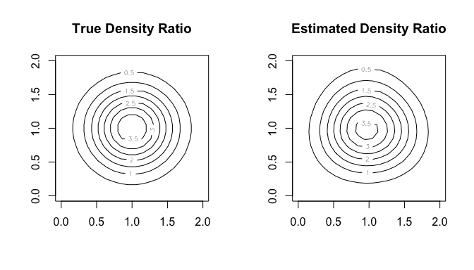
The densratio package has been used in several research papers, including: