The goal of detectnorm is to speculate the skewness and
kurtosis based on the Beta and truncated normal distribution. When
conducting a meta-analysis for two independent groups, we generally
retrieved very limited statistics from primary studies, and it is hard
to access the raw data. However, the non-normality of raw data could
influence the meta-analytic results greatly (Sun & Cheung, 2020).
This package allows meta-analysis researchers to speculate the skewness
and kurtosis of the raw data, even without the raw data. Instead of
normal distribution, if the researcher believes the population
distribution is non-normal, then beta-distribution could be a good
choice. If the researcher believes the population distribution is normal
but truncated by the measuring ability of the instrument, then truncated
normal distribution is a good option. The package provides not only the
skewness and kurtosis estimates but also the figures to visualize them.
Now, this package could work directly with the standardized mean
difference for two independent groups. It also works for one group of
data.
A good start to understand the problems of non-normality in primary studies on meta-analytic results is the following paper:
Sun, R. W., & Cheung, S. F. (2020). The influence of nonnormality from primary studies on the standardized mean difference in meta-analysis. Behavior Research Methods, 52(4), 1552-1567.
You can install the official version within R with:
install.packages("detectnorm")You can also install the development version of
detectnorm from GitHub
with:
# install.packages("devtools")
devtools::install_github("irissun/detectnorm")This is a basic example which shows you how to solve a common problem:
For one study if you assumed non-normal distribution in population:
library(detectnorm)
# Situations using beta distributions
set.seed(32411)
#Using Fleishman's method to generate non-normal data
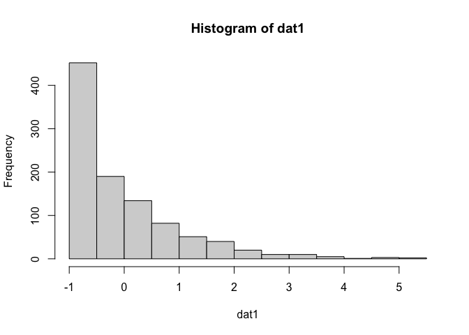
dat1 <- rnonnorm(n = 1000, mean = 0, sd = 1, skew = 2, kurt = 5)$dat
hist(dat1)
psych::describe(dat1)
#>    vars    n  mean sd median trimmed  mad   min  max range skew kurtosis   se
#> X1    1 1000 -0.01  1  -0.38    -0.2 0.63 -0.84 5.31  6.15 1.88     4.16 0.03
#Suppose we don't know about the raw data
result <- desbeta(vmean = mean(dat1), vsd = sd(dat1),lo = min(dat1), hi = max(dat1), showFigure = TRUE, rawdata = dat1)
#> [1] "mean is -0.0125212643739019"
#> [1] "sd is 0.999848046282588"
#> [1] "min. is -0.839243624241584"
#> [1] "max. is 5.31239864959992"
result
#> $dat
#>       alpha     beta      mean        sd skewness kurtosis
#> 1 0.4574073 2.946161 0.1343905 0.1625335 1.665152 2.572622
#>
#> $fig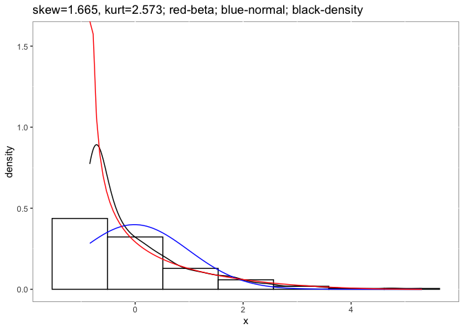
For one study if you assumed normal distribution in population with truncated by the measurements:
library(detectnorm)
#Truncated normal distribution
set.seed(34120)
dat2 <- truncnorm::rtruncnorm(n = 1000, a = 0, b = 14, mean = 4, sd = 3)
psych::describe(dat2)
#>    vars    n mean   sd median trimmed  mad  min   max range skew kurtosis   se
#> X1    1 1000 4.62 2.64   4.43    4.48 2.76 0.01 13.79 13.78 0.48    -0.13 0.08
destrunc(vmean=mean(dat2), vsd=sd(dat2), lo=0, hi=14, rawdata = dat2, showFigure = TRUE)
#> [1] "mean is 4.62042980360421"
#> [1] "sd is 2.63886011983622"
#> [1] "min. is 0"
#> [1] "max. is 14"
#> $dat
#>      pmean     psd      tm     tsd  skewness  kurtosis
#> 1 4.002982 3.15366 4.62043 2.63886 0.4499033 -0.252266
#>
#> $fig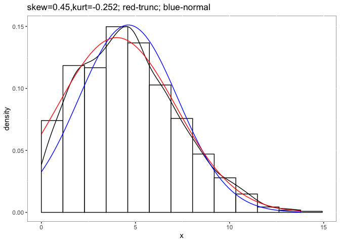
For one meta-analysis of two independent groups. It is very similar
to the requirements for package metafor only you need to
add one or two columns for each group about the possible minimum and
maximum of the data. It will add information including:
g1_alpha, g1_beta,
g2_alpha, and g2_beta are the shape parameters
of beta distributions;
g1_mean, g1_sd, g2_mean,
g2_sd are the means and standard deviations of the standard
beta distribution (ranged from 0 to 1);
g1_skewness, g1_kurtosis,
g2_skewness, and g2_kurtosis are the skewness
and kurtosis of the two groups.
In this example, it has contained the empirical skewness
skew1 and skew2, which are calculated from raw
data.
library(detectnorm)
# examine the meta-analysis dataset by simulating extremely non-normal distribution
# population mean1 = 1, mean2 = 1.5, sd1 = sd2=1, skewness1 = 4, kurtosis2 = 2, skewness2=-4, kurtosis2=2
data("beta_mdat")
beta1 <- detectnorm(m1i = m1,sd1i = sd1,n1i = n1, hi1i = hi1,lo1i = lo1,m2i = m2,sd2i = sd2,n2i = n2, hi2i = hi2,lo2i=lo2,distri = "beta", data = beta_mdat)
head(beta1)
#>   study  n1        m1       sd1       lo1      hi1  n2       m2       sd2
#> 1     1 160 1.0259203 0.8995642 0.2083603 5.578894 160 1.430021 1.0598447
#> 2     2  34 1.1528144 1.1367622 0.2123795 4.932592  34 1.408080 0.9296092
#> 3     3  57 0.9959042 0.8760782 0.2089018 3.443021  57 1.508927 1.0423997
#> 4     4 155 0.9480018 0.8828343 0.2082652 3.934242 155 1.443682 0.9198336
#> 5     5 149 1.1162247 1.0968963 0.2081850 5.613920 149 1.444312 1.0826183
#> 6     6 132 1.0418582 0.8946956 0.2082168 4.301961 132 1.554712 0.7932896
#>         lo2      hi2    skew1     skew2  g1_alpha  g1_beta   g1_mean     g1_sd
#> 1 -3.177617 2.274204 1.788613 -2.230054 0.5480186 3.051904 0.1522307 0.1674999
#> 2 -1.296619 2.271800 1.655752 -1.232207 0.3488177 1.401962 0.1992357 0.2408286
#> 3 -2.287307 2.274883 1.292354 -1.627030 0.3672680 1.141989 0.2433436 0.2708861
#> 4 -2.072880 2.274900 1.530104 -1.560090 0.3641696 1.470115 0.1985349 0.2369403
#> 5 -4.294234 2.274901 1.541182 -2.244364 0.4022054 1.992201 0.1679771 0.2029134
#> 6 -2.987192 2.273312 1.508507 -2.096631 0.4877450 1.907413 0.2036379 0.2185519
#>   g1_skewness g1_kurtosis g2_alpha   g2_beta   g2_mean     g2_sd g2_skewness
#> 1    1.483046   1.8901609 2.081468 0.3813533 0.8451559 0.1944020   -1.591348
#> 2    1.331854   0.8377363 1.291009 0.4122712 0.7579545 0.2605101   -1.069528
#> 3    1.079966   0.0309162 1.394623 0.2813890 0.8321080 0.2284867   -1.581618
#> 4    1.327314   0.8548620 1.985434 0.4693019 0.8088177 0.2115640   -1.310686
#> 5    1.489420   1.5984400 2.678914 0.3877426 0.8735618 0.1648038   -1.789508
#> 6    1.234109   0.7489875 3.614481 0.5718672 0.8633971 0.1508011   -1.558126
#>   g2_kurtosis
#> 1  2.00489688
#> 2  0.07531228
#> 3  1.66667585
#> 4  1.00447883
#> 5  3.02270945
#> 6  2.29997673
#compare the sample skewness and estimated skewness using beta distribution
mean(beta1$skew1)#sample skewness calculated from the sample in group 1
#> [1] 1.687593
mean(beta1$g1_skewness) #estimated using beta in group 1
#> [1] 1.384237
mean(beta1$skew2) #sample skewness calculated from the sample in group 2
#> [1] -1.687784
mean(beta1$g2_skewness)#estimated using beta in group 2
#> [1] -1.411431library(detectnorm)
data("trun_mdat")
head(trun_mdat)
#> study n1 m1 sd1 lo1 hi1 n2 m2 sd2
#> 1 1 199 1.297501 0.8203794 0.0061563102 3.611959 199 1.572915 0.9002734
#> 2 2 77 1.325658 0.7750929 0.0231261133 2.889290 77 1.597681 0.8782761
#> 3 3 166 1.212825 0.7460359 0.0158618581 3.607032 166 1.612654 0.8441273
#> 4 4 120 1.230577 0.7888702 0.0030294235 3.443851 120 1.598539 0.8776627
#> 5 5 175 1.279821 0.7477283 0.0002848415 3.409888 175 1.612636 0.8426223
#> 6 6 47 1.310062 0.8904328 0.0088877511 3.729032 47 1.613387 0.8375352
#> lo2 hi2 skew1 skew2
#> 1 0.02056929 3.654732 0.4925754 0.31062433
#> 2 0.01601133 3.591504 0.3189877 0.31978670
#> 3 0.02598881 3.944059 0.8236975 0.41657818
#> 4 0.05609411 3.563257 0.5632971 0.17020660
#> 5 0.01150730 3.784293 0.4826745 0.20444248
#> 6 0.04276128 3.137731 0.7678702 -0.02343749
trun1 <- detectnorm(m1i = m1,sd1i = sd1,n1i = n1, hi1i = 4,lo1i = 0,m2i = m2,sd2i = sd2,n2i = n2, hi2i = 4,lo2i= 0,distri = "truncnorm", data = trun_mdat)
mean(trun1$skew1)#sample skewness calculated from the sample in group 1
#> [1] 0.5142782
mean(trun1$g1_skewness)#estimated using truncnorm in group 1
#> [1] 0.5198264
mean(trun1$skew2)#sample skewness calculated from the sample in group 2
#> [1] 0.2023012
mean(trun1$g2_skewness)#estimated using truncnorm in group 2
#> [1] 0.254666