![]()

ecic estimates a changes-in-changes model with multiple
periods and cohorts as suggested in Athey and Imbens (2006).
Changes-in-changes is a generalization of the difference-in-differences
approach, estimating a treatment effect for the entire distribution
instead of averages.
Athey and Imbens (2006) show how to extend the model to multiple periods and cohorts, analogously to a two-way fixed-effects model for averages. This package implements this, calculating standard errors via bootstrap and plotting results, aggregated or in an event-study-style fashion.
ecic is available on CRAN using:
install.packages("ecic")You can install the newest version from GitHub:
# install.packages("remotes")
remotes::install_github("frederickluser/ecic")Let’s look at a short example how to use the package. First, load some simulated sample data.
library(ecic)
data(dat, package = "ecic")

head(dat)
#>  countyreal  first.treat   year time_to_treat   lemp
#>       <int>        <int>  <int>         <int>  <dbl>
#>           3        1980    1980             0   2.21
#>           3        1980    1981             1   3.33
#>           3        1980    1982             2   3.67
#>           5        1980    1980             0   2.77
#>           5        1980    1981             1   3.88
#>           5        1980    1982             2   3.80
Then, the function ecic estimates the
changes-changes-model:
# Estimate the model
mod =
  ecic(
    yvar  = lemp,         # dependent variable
    gvar  = first.treat,  # group indicator
    tvar  = year,         # time indicator
    ivar  = countyreal,   # unit ID
    dat   = dat,          # dataset
    boot  = "weighted",   # bootstrap proceduce ("no", "normal", or "weighted")
    nReps = 10            # number of bootstrap runs
    )
The input gvar denotes the period in which this
individual receives the treatment. mod contains for every
bootstrap run the point-estimates. The function summary
then combines all bootstrap runs to a quantile treatment effect and adds
standard errors:
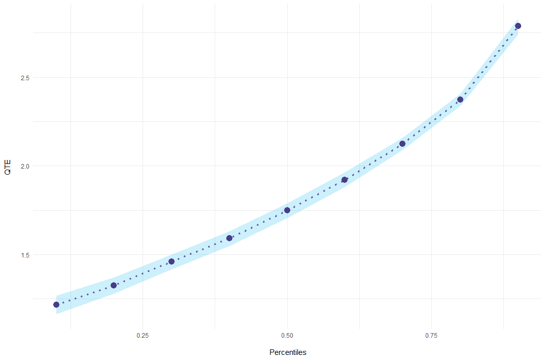
mod_res = summary(mod)

#> perc    coefs         se
#>  0.1 1.215531 0.02670761
#>  0.2 1.324130 0.02310521
#>  0.3 1.458270 0.02105119
#>  0.4 1.590848 0.02128534
#>  0.5 1.747296 0.02098057
#>  0.6 1.921818 0.02135982
#>  0.7 2.124138 0.01802972
#>  0.8 2.372483 0.01799869
#> 0.9 2.787395 0.02241811Finally, results can be plotted using ecic_plot.
ecic_plot(mod_res)
The package also allows to report event-study-style results
of the effect. To do so, simply add the es = T argument to
the estimation and summary will report effects for every
event period.
# Estimate the model
mod =
  ecic(
    yvar  = lemp,         # dependent variable
    gvar  = first.treat,  # group indicator
    tvar  = year,         # time indicator
    ivar  = countyreal,   # unit ID
    dat   = dat,          # dataset
    es    = T,            # report an event study
    boot  = "weighted",   # bootstrap proceduce ("no", "normal", or "weighted")
    nReps = 10            # number of bootstrap runs
    )

# report results for every event period
mod_res = summary(mod)

#> [[1]]
#> perc es     coefs         se
#>  0.1  0 0.9175263 0.02924326
#>  0.2  0 0.9675225 0.02508082
#>  0.3  0 0.9959150 0.02116782
#>  0.4  0 1.0388312 0.02373263
#>  0.5  0 1.0992322 0.02558309
#>  0.6  0 1.1496203 0.03078493
#>  0.7  0 1.2049797 0.03654320
#>  0.8  0 1.2519476 0.03291178
#>  0.9  0 1.3616626 0.01765538

#> [[2]]
#> perc es    coefs          se
#>  0.1  1 2.393816 0.022273736
#>  0.2  1 2.386941 0.020039276
#>  0.3  1 2.423415 0.017145110
#>  0.4  1 2.452259 0.017982620
#>  0.5  1 2.484616 0.009979006
#>  0.6  1 2.525388 0.012816760
#>  0.7  1 2.575615 0.015196499
#>  0.8  1 2.630959 0.019570320
#>  0.9  1 2.730742 0.024796025
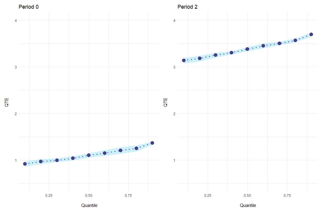
#> [...]In addition to a standard plot showing everything at once,
event-study results can be plotted for every period individually with
the option es_type = "for_periods".
ecic_plot(
    mod_res,
    periods_plot = c(0, 2),   # which periods you want to show
    es_type = "for_periods",  # plots by period
    ylim = c(.5, 4)           # same y-axis
    )
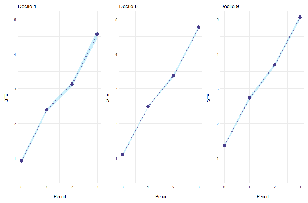
Alternatively, es_type = "for_quantiles" generates one
plot for every quantile of interest.
ecic_plot(
    mod_res,
    periods_plot = c(.1, .5, .9), # which quantiles you want to show
    es_type = "for_quantiles",    # plots by period
    ylim = c(.5, 5)               # same y-axis
    )
For every treated cohort, we observe the distribution of the potential outcome \(Y(1)\). In the case of two groups / cohorts and two periods, Athey and Imbens (2006) show how to construct the counterfactual \(Y(0)\). This extends to the case with multiple cohorts and periods, where every not-yet-treated cohort is a valid comparison group. Hence, every combination of treated and not-yet-treated cohorts with a common pre-treatment period estimates in theory the quantile treatment effect. Then, I simply want to average them.
Yet, since it is not allowed to simply average quantile treatment effects, we must first store the empirical CDF of \(Y(1)\) and \(Y(0)\) for every two-by-two case. Next, I aggregate all estimated CDFs to get the plug-in estimates of \(Y(1)\) and \(Y(0)\), weighting for the cohort sizes. Finally, I invert them to get the quantile function and compute the quantile treatment effect as in the standard case.
Note that it is impossible to estimate a quantile treatment effect
for units treated in the first (no pre-treatment period) and last period
(no comparison cohort). In addition, the default value of
nMin skips small cohorts (default nMin = 40)
as we need more observations to estimate quantile treatment effects
compared to an average effect.
Technically, ecic generates a grid over the dependent
variable and imputes all empirical CDFs for every unique value of
yvar. You can (cautiously) speed up the imputation by
rounding the dependent variable to n_digits.
I calculate standard errors by bootstrap. I resample with replacement
the entire dataset and estimate \(Y(1)\) and \(Y(0)\) nRep times (default
nReps = 1). Bootstrap can either be computed through
replacement over the entire dataset (with boot = "normal")
or you can weight by cohort sizes (with boot = "weighted")
if you worry, for example, about small cohorts. This part can be
parallelized by setting nCores > 1, speeding up the
computation at the cost of additional overhead to load the cores.
progress_bar prints the progress of the bootstrapping by
default. Alternatively, the option progress_bar = "cli"
also shows estimated running time, but requires the cli
package to be installed.