eeptools is an R package that seeks to make it easier
for analysts at state and local education agencies to analyze and
visualize their data on student, school, and district performance. By
putting simple wrappers around a number of R functions,
eeptools strives to make many common tasks simpler and less
prone to error specific to analysis of education data.
eeptools provides three new datasets of interest to
education researchers. These datasets are also used in the R Bootcamp for
Education Analysts
library(eeptools)
#> Loading required package: ggplot2
data("stuatt")
head(stuatt)
#>   sid school_year male race_ethnicity birth_date first_9th_school_year_reported
#> 1   1        2004    1              B      10869                           2004
#> 2   1        2005    1              H      10869                           2004
#> 3   1        2006    1              H      10869                           2004
#> 4   1        2007    1              H      10869                           2004
#> 5   2        2006    0              W      11948                             NA
#> 6   2        2007    0              B      11948                             NA
#>   hs_diploma      hs_diploma_type hs_diploma_date
#> 1          0
#> 2          0
#> 3          0
#> 4          0
#> 5          1     Standard Diploma        6/5/2008
#> 6          1 College Prep Diploma       5/24/2009
The stuatt, student attributes, dataset is provided from
the Strategic
Data Project Toolkit for Effective Data Use. This dataset is useful
for learning how to clean data in R and how to aggregate and summarize
individual unit-record data into group-level data.
data(stulevel)
head(stulevel)
#>     X school  stuid grade schid dist white black hisp indian asian econ female
#> 1  44      1 149995     3   495  105     0     1    0      0     0    0      0
#> 2  53      1  13495     3   495   45     0     1    0      0     0    1      0
#> 3 116      1 106495     3   495   45     0     1    0      0     0    1      0
#> 4 244      1  45205     3   205   15     0     1    0      0     0    1      0
#> 5 274      1 142705     3   205   75     0     1    0      0     0    1      0
#> 6 276      1  14995     3   495  105     0     1    0      0     0    1      0
#>   ell disab sch_fay dist_fay luck   ability    measerr      teachq year attday
#> 1   0     0       0        0    0  87.85405  11.133264 39.09024712 2000    180
#> 2   0     0       0        0    1  97.78756   6.822394  0.09848192 2000    180
#> 3   0     0       0        0    0 104.49303  -7.856159 39.53885270 2000    160
#> 4   0     0       0        0    1 111.67151 -17.574152 24.11612277 2000    168
#> 5   0     0       0        0    0  81.92539  52.983338 56.68061304 2000    156
#> 6   0     0       0        0    0 101.92904  22.604145 71.62196655 2000    157
#>   schoolscore district schoolhigh schoolavg schoollow   readSS   mathSS
#> 1    29.22427        3          0         1         0 357.2865 387.2803
#> 2    55.96326        3          0         1         0 263.9046 302.5724
#> 3    55.96326        3          0         1         0 369.6722 365.4614
#> 4    55.96326        3          0         1         0 346.5957 344.4964
#> 5    55.96326        3          0         1         0 373.1254 441.1581
#> 6    55.96326        3          0         1         0 436.7607 463.4033
#>       proflvl race
#> 1       basic    B
#> 2 below basic    B
#> 3       basic    B
#> 4       basic    B
#> 5       basic    B
#> 6  proficient    B
The stulevel dataset is a simulated student-level
longitudinal record. It contains student and school level attributes and
is useful for practicing evaluating longitudinal analyses of student
unit-record data.
data("midsch")
head(midsch)
#>   district_id school_id subject grade n1   ss1 n2   ss2 predicted  residuals
#> 1          14       130    math     4 44 433.1 40 463.0  468.7446 -5.7445937
#> 2          70        20    math     4 18 443.0 20 477.2  476.4765  0.7235053
#> 3         112        80    math     4 86 445.4 94 472.6  478.3509 -5.7508949
#> 4         119        50    math     4 95 427.1 94 460.7  464.0586 -3.3585931
#> 5         147        60    math     4 27 424.2 27 458.7  461.7937 -3.0936928
#> 6         147       125    math     4 17 423.5 26 463.1  461.2470  1.8530072
#>       resid_z     resid_t       cooks test_year     tprob flagged_t95
#> 1 -0.59189645 -0.59170988 0.000171271      2007 0.2787298           0
#> 2  0.07455731  0.07452135 0.000003510      2007 0.4706873           0
#> 3 -0.59266905 -0.59248250 0.000244921      2007 0.2774827           0
#> 4 -0.34605798 -0.34591020 0.000059900      2007 0.3650957           0
#> 5 -0.31877383 -0.31863490 0.000054100      2007 0.3762745           0
#> 6  0.19093568  0.19084643 0.000019800      2007 0.4250936           0
The midsch dataset contains an analysis on abnormality
in school average assessment scores. It contains observed and predicted
values of aggregated test scores at the school level for a large
midwestern state.
For analysts using unit-record data of some type, there are several
calc functions which automate common tasks including
calculating ages (age_calc), grade retention
(retained_calc), and student mobility
(moves_calc).
age_calc(dob = as.Date('1995-01-15'), enddate = as.Date('2003-02-16'),
         units = "years")
#> [1] 8.087671
age_calc(dob = as.Date('1995-01-15'), enddate = as.Date('2003-02-16'),
         units = "months")
#> [1] 97.03571
age_calc(dob = as.Date('1995-01-15'), enddate = as.Date('2003-02-16'),
         units = "days")
#> Time difference of 2954 days
age_calc also now properly accounts for leap years and
leap seconds by default.
retained_calc takes a vector of student identifiers and
a vector of grades and checks whether or not the student was retained in
the grade level specified by the user. It returns a data.frame of all
students who could have been retained and a yes or no indicator of
whether they were retained.
x <- data.frame(sid = c(101, 101, 102, 103, 103, 103, 104, 105, 105, 106, 106),
                 grade = c(9, 10, 9, 9, 9, 10, 10, 8, 9, 7, 7))
retained_calc(df = x, sid = "sid", grade = "grade", grade_val = 9)
#>   sid retained
#> 1 101        N
#> 2 102        N
#> 3 103        Y
#> 4 105        N
retained_calc is intended to be used after you have
processed your data as it does not take into account time or sequence
other than the order in which the data is passed to it.
moves_calc is intended to identify based on enrollment
dates whether a student experienced a school move within a school
year.
df <- data.frame(sid = c(rep(1,3), rep(2,4), 3, rep(4,2)),
                   schid = c(1, 2, 2, 2, 3, 1, 1, 1, 3, 1),
                   enroll_date = as.Date(c('2004-08-26',
                   '2004-10-01', '2005-05-01', '2004-09-01',
                   '2004-11-03', '2005-01-11', '2005-04-02',
                   '2004-09-26', '2004-09-01','2005-02-02'), format='%Y-%m-%d'),
                   exit_date = as.Date(c('2004-08-26', '2005-04-10',
                    '2005-06-15', '2004-11-02', '2005-01-10',
                    '2005-03-01', '2005-06-15', '2005-05-30',
                    NA, '2005-06-15'), format='%Y-%m-%d'))

moves <- moves_calc(df, sid = "sid", schid = "schid", enroll_date = "enroll_date",
                    exit_date = "exit_date")
moves
#>   sid moves
#> 1   1     4
#> 2   2     4
#> 3   3     2
#> 4 4 NAAnother set of key functions in the package are to make basic data
manipulation easier. One thing users of other statistical packaegs may
miss when using R is a convenient function for determining the
mode of a vector. The statamode function is
designed to do just that. statamode works with numeric,
character, and factor data types. It also includes various options for
how to deal with a tie demonstrated below.
vecA <- c(1, 2, 3, 4, 5, 6, 7, 8, 9, 10)
statamode(vecA, method = "stata")
#> [1] "."
vecB <- c(1, 1, 1, 3:10)
statamode(vecB, method = "last")
#> [1] 1
vecC <- c(1, 1, 1, NA, NA, 5:10)
statamode(vecC, method = "last")
#> [1] 1
vecA <- c(LETTERS[1:10]); vecA <- factor(vecA)
statamode(vecA, method = "last")
#> [1] J
#> Levels: J
vecB <- c("A", "A", "A", LETTERS[3:10]); vecB <- factor(vecB)
statamode(vecB, method = "last")
#> [1] A
#> Levels: A
vecA <- c(LETTERS[1:10])
statamode(vecA, method = "sample")
#> [1] "B"
vecB <- c("A", "A", "A", LETTERS[3:10])
statamode(vecB, method = "stata")
#> [1] "A"
vecC <- c("A", "A", "A", NA, NA, LETTERS[5:10])
statamode(vecC, method = "stata")
#> [1] "A"
There are a number of functions to save you keystrokes like
defac for converting a factor to a character,
makenum for turning a factor variable into a numeric
variable, max_mis for taking the maximum of a vector of
numerics and ignoring any NAs (useful for inclusion in
do.call or apply constructions).
remove_char allows you to quickly gsub out a
specific character from a string vector such as an * or
.... decomma is a somewhat specialized version
of this for processing data where numerics are written with commas.
nth_max allows you to identify the 2nd, 3rd, etc. maximum
value in a vector.
eeptools includes ways to simplify the use of regression
analyses tools recommended by Gelman and Hill 2006 through the
gelmansim function, which itself is a wrapper for the
arm::sim() function.
require(MASS)
#> Loading required package: MASS
#Examples of "sim"
set.seed (1)
J <- 15
n <- J*(J+1)/2
group <- rep (1:J, 1:J)
mu.a <- 5
sigma.a <- 2
a <- rnorm (J, mu.a, sigma.a)
b <- -3
x <- rnorm (n, 2, 1)
sigma.y <- 6
y <- rnorm (n, a[group] + b*x, sigma.y)
u <- runif (J, 0, 3)
dat <- cbind (y, x, group)
# Linear regression
dat <- as.data.frame(dat)
dat$group <- factor(dat$group)
M3 <- glm (y ~ x + group, data=dat)
cases <- expand.grid(x = seq(-2, 2, by=0.1),
                     group=seq(1, 14, by=2))
cases$group <- factor(cases$group)
sim.results <- gelmansim(mod = M3, newdata = cases, n.sims=200, na.omit=TRUE)
head(sim.results)
#>      x group      yhats   yhatMin  yhatMax
#> 1 -2.0     1  1.1071284 -6.348896 8.202628
#> 2 -1.9     1  0.6736463 -7.511567 8.400011
#> 3 -1.8     1  1.1224105 -6.679137 8.144215
#> 4 -1.7     1 -0.4248225 -8.419041 6.984633
#> 5 -1.6     1  0.1310932 -7.320700 9.293344
#> 6 -1.5     1 -0.6902903 -8.019434 7.595934
There is also a ggplot2 version of plot.lm
included:
data(mpg)
mymod <- lm(cty~displ + cyl + drv, data=mpg)
autoplot(mymod)
#> `geom_smooth()` using formula = 'y ~ x'
#> `geom_smooth()` using formula = 'y ~ x'
#> `geom_smooth()` using formula = 'y ~ x'
#> `geom_smooth()` using formula = 'y ~ x'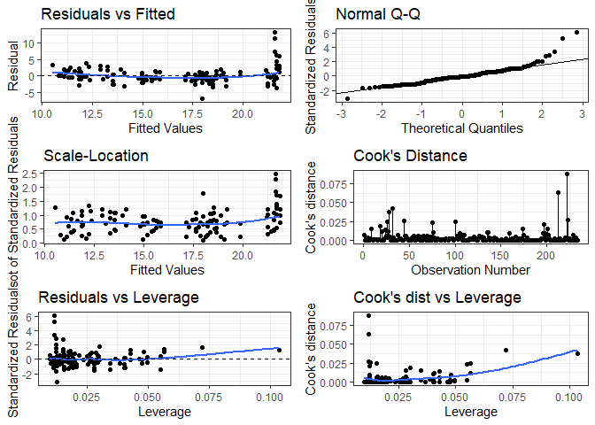
Finally, there is a convenient method for creating labeled mosaic plots.
sampDat <- data.frame(cbind(x=seq(1,3,by=1), y=sample(LETTERS[6:8], 60,
                                                        replace=TRUE)),
                        fac=sample(LETTERS[1:4], 60, replace=TRUE))
varnames<-c('Quality','Grade')
crosstabplot(sampDat, "y", "fac", varnames = varnames,  label = TRUE,
             title = "Crosstab Plot", shade = FALSE)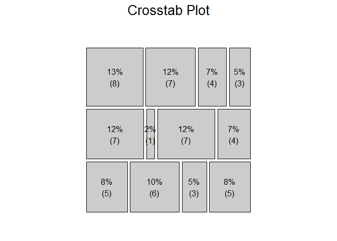
Review the Contributor Guide for specific directions and tips on how to get involved.
eeptools is intended to be a useful project for the
education analytics community. Contributions are welcomed. Please note
that this project is released with a Contributor
Code of Conduct. By participating in this project you agree to abide
by its terms.