Authors: Amine Gassem, Irina Baltcheva, Christian Bartels, Souvik Bhattacharya, Thomas Dumortier, Matthew Fidler, Seid Hamzic, Inga Ludwig, Ines Paule, Didier Renard, Bruno Bieth
![]()
![]()
ggPMX is an open-source R package freely available on CRAN since April 2019. It generates standard diagnostic plots for mixed effect models used in pharmacometric activities. The package builds on the R-package ggplot2 and aims at providing a workflow that is consistent, reproducible and efficient, resulting in high quality graphics ready-to-use in submission documents and publications. Intuitive functions and options allow for optimal figure customization and graphics stratification. ggPMX enables straightforward generation of PDF, Word or PNG output files that contain all diagnostic plots for keeping track of modeling results. The package is currently compatible with Monolix versions 2016 and later, NONMEM version 7.2 and later and nlmixr.
Using simple syntax, the toolbox produces various goodness-of-fit diagnostics such as: - residual- and empirical Bayes estimate (EBE)-based plots, - distribution plots, - prediction- and simulation-based diagnostics (visual predictive checks).
ggPMX creates plot objects which can be further customized and extended using the extensive ggplot2 syntax.
In addition, shrinkage and summary parameters tables can be also produced. By default, the PDF- or Word-format diagnostic report contains essential goodness-of-fit plots. However, these can be adapted to produce different sets of diagnostics as desired by the user, and any of the plots may be customized individually. The types of supported customizations include modifications of the graphical parameters, labels, and various stratifications by covariates.
# Either install from CRAN
install.packages("ggPMX")
# Or the development version from GitHub:
# install.packages("devtools")
devtools::install_github("ggPMXdevelopment/ggPMX")Once ggPMX is installed, you can test if everything is working well. If successful you should see a plot created after the following build-in example.
library(ggPMX)
ctr <- theophylline()
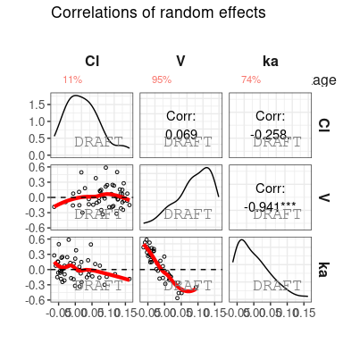
ctr %>% pmx_plot_eta_matrix()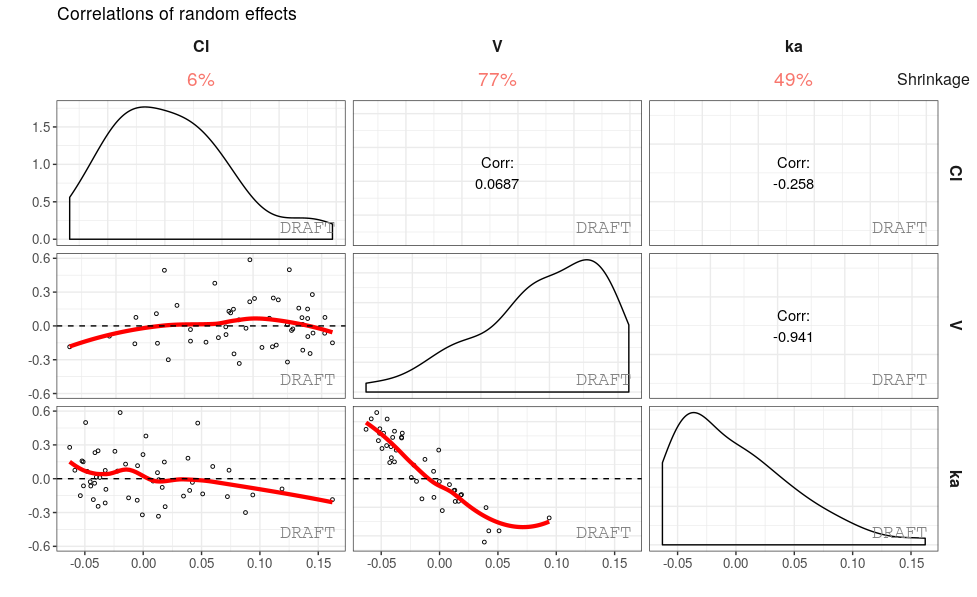
ggPMX is now ready for inputs and enhancements by the pharmacometric community. - Please use package issues to fill in your feedback.
The ggPMX package generates standard diagnostic plots
and tables for mixed effect models used in Pharmacometric (PMX)
activities. The tool is built upon the ggplot2 package and supports
models developped with Monolix, NONMEM and nlmixr software. The current
release (1.2) supports models fitted with Monolix versions 2016 and
later, NONMEM version 7.2 and later and nlmixr.
The package aims to provide a workflow that is consistent, efficient and which results in high quality graphics ready to use in official documents and reports. The package allows a high degree of flexibility and customization, yet providing an acceptable default setting. The package also allows to fully automate plots and report generation.
The general context is the analysis of mixed effect models fitted to data. ggPMX was developed in the framework of Pharmacometric activities, in which case the model is a population pharmacokinetic (PK) and/or pharmacodynamic (PD) model and the data is clinical or pre-clinical PK and/or PD data.
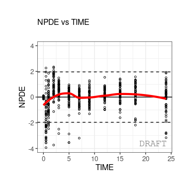
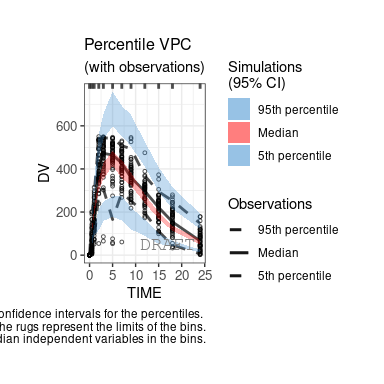
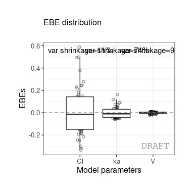
In the context of model building, evaluation and qualification, it is good practice to assess the goodness-of-fit of models by inspecting (qualitatively and quantitatively) a set of graphs that indicate how well the model describes the data. Several types of diagnostic plots allow to evaluate a mixed effects model fit, the most common being:
The following figures are examples of diagnotic plots.
This document introduces the ggPMX functionalities and syntax.
The high level architecture is represented in the figure below. The key components of the package are the following:
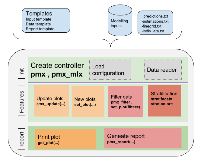
The package is coded using object-oriented programming meaning that information is encoded in objects. The user can change or print the content of objects via functions. Such an implementation allows to have code that is modular and easily customizable.
The typical workflow of ggPMX is as follows:
The most important task for the user is the Controller creation. This step requires careful consideration because it involves different options according to the type of model (PK or PKPD) and software (Monolix, NONMEM or nlmixr) used for model fitting. The next section describes the Controller creation for the different possible cases.
Once the Controller is created, it implicitly calls the Reader and creates the diagnostic plots. The user can then generate the graphs by calling pre-defined functions. The same syntax is used independent of the model structure (PK or PKPD model) and of the fitting software.
The Reporter creates one report per endpoint, i.e., one report for PK and one for each PD endpoint.
For the sake of this document, three types of datasets are defined.
A diagnostic session starts with the creation of a Controller. The
Controller is the “user interface” of the package and allows to conrol
all possible options. It is a container that stores configuration fields
(model- and input data-related information), datasets and plots. It can
be used as a reference object in which the user can see the names of the
exisitng plots, the names of the ggPMX datasets, etc. The
syntax of the Controller creation differs depending on the software used
for model fitting and on the number of model endpoints (or outputs).
This section presents different cases of Controller creation. For
simplicity, the case of models with one single output is presented
first, then generalized to several outputs. ## Single-endpoint
models
In general, models with only one endpoint (or output) are mostly PK models, but these could also be k-PD models.
To illustrate ggPMX functionalities, the single-endpoint
built-in model called theophylline is used hereafter.
The theophylline population PK example has the
following characteristics:
The input modeling dataset has the following columns:
#>   ID TIME  AMT   Y EVID WT0 AGE0 SEX STUD
#> 1  1  0.0 2000   0    1  87   73   1    1
#> 2  1  0.5    0 130    0  87   73   1    1
#> 3  1  1.0    0 228    0  87   73   1    1
#> 4  1  2.0    0 495    0  87   73   1    1
#> 5  1  3.0    0 484    0  87   73   1    1
#> 6  1  5.0    0 479    0  87   73   1    1
Note that the DVID (or CMT/YTYPE) column is missing, but since this is a single-endpoint model, it is not necessary in that case.
The Contoller creation is wrapped in a function called “theophylline()” for quick reference:
ctr <- theophylline()pmx_mlx()The controller initialization using the Monolix controller
pmx_mlx(), which is a wrapper function for
pmx() with sys="mlx" (See Appendix A).
theophylline_path <- file.path(system.file(package = "ggPMX"), "testdata", "theophylline")
work_dir          <- file.path(theophylline_path, "Monolix")
input_data_path   <- file.path(theophylline_path, "data_pk.csv")

ctr <- pmx_mlx(
  directory = work_dir,
  input     = input_data_path,
  dv        = "Y"
)####pmx_mlxtran()
The controller initialization can be simplified by using the Monolix
controller pmx_mlxtran(). This function parses the mlxtran
file of a Monolix project and assigns automatically the different fields
necessary to the Controller creation. The only mandatory argument is
file_name, the path to the mlxtran file.
mlxtran_path <- file.path(system.file(package = "ggPMX"),
                          "testdata", "1_popPK_model", "project.mlxtran")

ctr <- pmx_mlxtran(file_name = mlxtran_path)
The user can verify the content of the Controller and how parameters are assigned by printing it.
pmx_nm()The controller initialization using the NONMEM controller
pmx_nm() is based on reading functions of the xpose
package. It is highly recommended (but not required) to use the “sdtab,
patab, cotab, catab” table naming convention followed by a run number
(e.g. sdtab001,cotab001) This will enable automatic recognition of
covariates. It is also recommended to name the model files accordingly
(e.g. run001.lst). In order to generate a VPC a simulation dataset is
required (see section about VPC)
For controller generation it is recommended to use the model file:
nonmem_dir <- file.path(system.file(package = "ggPMX"), "testdata","extdata")
ctr <- pmx_nm(
  directory = nonmem_dir,
  file     = "run001.lst"
)
or the run number. The standard prefix is “run”, however can be
specified using prefix
nonmem_dir <- file.path(system.file(package = "ggPMX"), "testdata","extdata")
ctr <- pmx_nm(
  directory = nonmem_dir,
  runno     = "001" #can be a string or a number
)pmx_nlmixr()It is simple to create a ggPMX controller for a nlmixr object using
pmx_nlmixr(). Using the theophylline example with a nlmixr
model we have:
one.cmt <- function() {
  ini({
    ## You may label each parameter with a comment
    tka <- 0.45 # Log Ka
    tcl <- 1 # Log Cl
    ## This works with interactive models
    ## You may also label the preceding line with label("label text")
    tv <- 3.45; label("log V")
    ## the label("Label name") works with all models
    eta.ka ~ 0.6
    eta.cl ~ 0.3
    eta.v ~ 0.1
    add.sd <- 0.7
  })
  model({
    ka <- exp(tka + eta.ka)
    cl <- exp(tcl + eta.cl)
    v <- exp(tv + eta.v)
    linCmt() ~ add(add.sd)
  })
}

fit <- nlmixr(one.cmt, theo_sd, est="saem", control=list(print=0))
The fit object is a nlmixr fit; You can read it into the
nlmixr controller by:
ctr <- pmx_nlmixr(fit,
                  vpc = FALSE ## VPC is turned on by default, can turn off
)The following are some optional arguments to the controller function
(for details of each option, see the corresponding section or use
?pmx_mlx, ?pmx_nm,
?pmx_nlmixr):
pmx_settings())
shared between all plotspmx_endpoint()) or integer
or charcater of the endpoint code (depends on the fitting software)Models with more than one endpoint (or output) are mostly PKPD models, but these could also be, for example, PK binding models in which there are measurements and predictions of both PK and its target.
ggPMX produces one diagnostics report per endpoint. As a consequence, the endpoint (if more than one) should be set at the time of the Controller creation in order to filter the observations dataset and to keep only the values corresponding to the endpoint of interest. There are two ways of dealing with endpoints, using pmx_endpoint() (only for Monolix), or a simplified syntax for endpoints which is supported by all software outputs.
To handle this, the user creates an “endpoint” object using the
function pmx_endpoint() having the following
attributes:
list(predictions="predictions1",finegrid ="finegrid1")To illustrate the Controller creation with multiple-endpoint models, a built-in PKPD example is used. The input dataset is called pk_pd.csv and has the following columns.
#>    id time amt  dv dvid   wt sex age
#> 1 100  0.0 100   .    3 66.7   1  50
#> 2 100  0.5   .   0    3 66.7   1  50
#> 3 100  1.0   . 1.9    3 66.7   1  50
#> 4 100  2.0   . 3.3    3 66.7   1  50
#> 5 100  3.0   . 6.6    3 66.7   1  50
#> 6 100  6.0   . 9.1    3 66.7   1  50
The dvid column contains values=3 for PK (first endpoint) and dose and =4 for PD (second endpoint). Monolix2016 outputs are found in folder RESULTS/ which contains predictions1.txt and finegrid1.txt for PK predictions, and predictions2.txt and finegrid2.txt for PD predictions. The Endpoint and Controller objects are created as follows:
pkpd_path       <- file.path(system.file(package = "ggPMX"), "testdata", "pk_pd")
pkpd_work_dir   <- file.path(pkpd_path, "RESULTS")
pkpd_input_file <- file.path(pkpd_path, "pk_pd.csv")

ep <- pmx_endpoint(
  code  = "4",
  label = "some_label",
  unit  = "some_unit",
  file.code = "2", # will use predictions2.txt and finegrig2.txt
  trans = "log10"
)

ctr <- pmx_mlx(
  directory = pkpd_work_dir,
  input     = pkpd_input_file,
  dv        = "dv",
  dvid      = "dvid",
  endpoint  = ep
)
#> use  predictions2.txt  as  model predictions file .
#> use finegrid2.txt as finegrid file .For NONMEM and nlmixr users, endpoint can be simply specified in the
controller creation by e.g. endpoint = 1
NONMEM
ctr <- pmx_nm(
  directory = nonmem_dir,
  file     = "run001.lst",
  endpoint = 1 ## select the first endpoint
  dvid = "DVID" ## use this column as observation id
)
nlmixr
ctr <- pmx_nlmixr(fit,
                  endpoint = 1 ## select the first endpoint
                  dvid = "DVID" ## use this column as observation id
)
Also for Monolix users, a simplified syntax for the Endpoint creation exists in the case where the endpoint code matches the files post-fixes (code=1 corresponds to predictions1.txt, code=2 corresponds to predictions2.txt). Instead of passing a pmxEndpoint object as argument of the Controller, the user can specify the numerical value corresponding to the YTYPE/CMT/DVID column.
pmx_mlx(
  dvid = "YTYPE", ## use this column as observation id
  endpoint = 1,   ## select the first endpoint
  ...)            ## other pmx parameters , config, input,etc..
Internally, a pmxEndpoint object will be created, and observations having YTYPE=x will be filtered.
When fitting a multiple-endpoint model, Monolix is known to rename endpoint variables to y1, y2. For controller creation to work it may necessary to reverse this renaming in the simulation file (e.g. y1 -> LIDV).
Besides the mandatory fields to initialize a Controller, the user can set optional parameters related to covariates. This feature is illustrated below with the Theophylline example.
theophylline_path <- file.path(system.file(package = "ggPMX"), "testdata", "theophylline")
work_dir          <- file.path(theophylline_path, "Monolix")
input_data_path   <- file.path(theophylline_path, "data_pk.csv")

ctr <- pmx_mlx(
  directory = work_dir,
  input     = input_data_path,
  dv        = "Y",
  cats      = c("SEX"),
  conts     = c("WT0", "AGE0"),
  strats    = c("STUD", "SEX")
)
Conts are the continuous covariates. Cats
are categorical covariates used in the model, whereas
strats are categorical variables that can be used for plot
stratification, but are not used as covariates in the model.
The covariates can be accessed using helper functions:
ctr %>% get_cats()
#> [1] "SEX"
ctr %>% get_conts()
#> [1] "WT0"  "AGE0"
ctr %>% get_strats()
#> [1] "STUD" "SEX"
ctr %>% get_covariates()
#> [1] "SEX" "WT0" "AGE0"The content of the Controller can be seen by printing it:
ctr
#>
#> pmx object:
#>
#>
#> |PARAM                |VALUE        |
#> |:--------------------|:------------|
#> |working directory    |theophylline |
#> |Modelling input file |data_pk.csv  |
#> |dv                   |Y            |
#> |dvid                 |DVID         |
#> |cats                 |SEX          |
#> |conts                |WT0,AGE0     |
#> |strats               |STUD,SEX     |
#>
#>
#> |data_name   |data_file       |data_label                                |
#> |:-----------|:---------------|:-----------------------------------------|
#> |predictions |predictions.txt |model predictions file                    |
#> |estimates   |estimates.txt   |parameter estimates file                  |
#> |eta         |indiv_eta.txt   |invidual estimates of random effects file |
#> |finegrid    |finegrid.txt    |finegrid file                             |
#> |input       |data_pk.csv     |modelling input                           |
#>
#>
#> |plot_name       |plot_type |
#> |:---------------|:---------|
#> |abs_iwres_ipred |SCATTER   |
#> |abs_iwres_time  |SCATTER   |
#> |iwres_ipred     |SCATTER   |
#> |iwres_time      |SCATTER   |
#> |iwres_dens      |PMX_DENS  |
#> |iwres_qq        |PMX_QQ    |
#> |npde_time       |SCATTER   |
#> |npde_pred       |SCATTER   |
#> |npde_qq         |PMX_QQ    |
#> |dv_pred         |SCATTER   |
#> |dv_ipred        |SCATTER   |
#> |individual      |IND       |
#> |eta_hist        |DIS       |
#> |eta_box         |DIS       |
#> |eta_matrix      |ETA_PAIRS |
#> |eta_cats        |ETA_COV   |
#> |eta_conts       |ETA_COV   |
#> |eta_qq          |PMX_QQ    |
It contains three tables:
The first table is the Controller configuration. The user can see the working directory, the input modeling dataset name, the dependent variable (DV) name and other fields related to the model (e.g., continuous and discrete covariates).
The second table lists the ggPMX datasets. The first
column (data_name) of this table contains the ggPMX name of
the dataset; the second column (data_file) contains the names of the
output modeling datasets (for example estimates.txt); in the third
column (data_label) contains the dataset description.
The third table provides the list of available plots in the Generator. It corresponds to Table .
The Controller is a container that stores all plots. To get the list
of plots, the function plot_names() is used:
ctr %>% plot_names()
#>  [1] "abs_iwres_ipred" "abs_iwres_time"  "iwres_ipred"     "iwres_time"
#>  [5] "iwres_dens"      "iwres_qq"        "npde_time"       "npde_pred"
#>  [9] "npde_qq"         "dv_pred"         "dv_ipred"        "individual"
#> [13] "eta_hist"        "eta_box"         "eta_matrix"      "eta_cats"
#> [17] "eta_conts"       "eta_qq"
An alternative way to display the names of the existing plots is by printing the content of the Controller as done above.
ggPMX provides a specialized function to create and
update each plot pmx_plot_xx() where xx is the
plot name from the list above.
Each plot type is a class of similar plots. ggPMX
defines the following plot types:
The following syntax allows to see which type of plot corresponds to which plot name:
ctr %>% plots()
#>           plot_name plot_type            plot_function
#>  1: abs_iwres_ipred   SCATTER pmx_plot_abs_iwres_ipred
#>  2:  abs_iwres_time   SCATTER  pmx_plot_abs_iwres_time
#>  3:     iwres_ipred   SCATTER     pmx_plot_iwres_ipred
#>  4:      iwres_time   SCATTER      pmx_plot_iwres_time
#>  5:      iwres_dens  PMX_DENS      pmx_plot_iwres_dens
#>  6:        iwres_qq    PMX_QQ        pmx_plot_iwres_qq
#>  7:       npde_time   SCATTER       pmx_plot_npde_time
#>  8:       npde_pred   SCATTER       pmx_plot_npde_pred
#>  9:         npde_qq    PMX_QQ         pmx_plot_npde_qq
#> 10:         dv_pred   SCATTER         pmx_plot_dv_pred
#> 11:        dv_ipred   SCATTER        pmx_plot_dv_ipred
#> 12:      individual       IND      pmx_plot_individual
#> 13:        eta_hist       DIS        pmx_plot_eta_hist
#> 14:         eta_box       DIS         pmx_plot_eta_box
#> 15:      eta_matrix ETA_PAIRS      pmx_plot_eta_matrix
#> 16:        eta_cats   ETA_COV        pmx_plot_eta_cats
#> 17:       eta_conts   ETA_COV       pmx_plot_eta_conts
#> 18: eta_qq PMX_QQ pmx_plot_eta_qqThe diagnostic plots of ggPMX are generated by calling the functions
pmx_plot_xx() where xx is a placeholder for
the plot name. The list of names of all available plots can be seen
via:
ctr %>% plot_names()
#>  [1] "abs_iwres_ipred" "abs_iwres_time"  "iwres_ipred"     "iwres_time"
#>  [5] "iwres_dens"      "iwres_qq"        "npde_time"       "npde_pred"
#>  [9] "npde_qq"         "dv_pred"         "dv_ipred"        "individual"
#> [13] "eta_hist"        "eta_box"         "eta_matrix"      "eta_cats"
#> [17] "eta_conts"       "eta_qq"          "pmx_vpc"
As a convention, when plots are described as ???Y vs. X???, it is meant that Y is plotted on the vertical axis and X on the horizontal axis.
As an example, a plot of individual weighted residuals (IWRES) versus time (with default settings) can be generated using a single-line code:
ctr %>% pmx_plot_iwres_time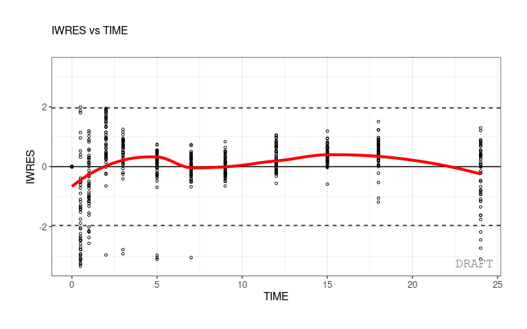
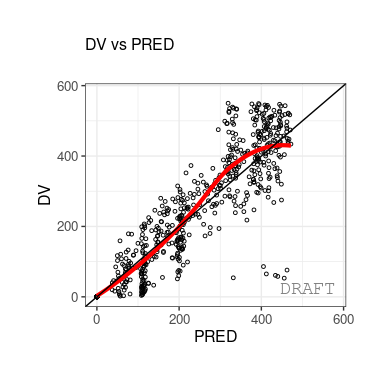
The complete list of available plots per plot type (given in parenthesis) is given below:
ctr %>% pmx_plot_dv_pred
ctr %>% pmx_plot_dv_ipred

ctr %>% pmx_plot_iwres_time
ctr %>% pmx_plot_npde_time

ctr %>% pmx_plot_iwres_ipred
ctr %>% pmx_plot_abs_iwres_ipred

ctr %>% pmx_plot_npde_predctr %>% pmx_plot_eta_hist
ctr %>% pmx_plot_eta_boxctr %>% pmx_plot_individual(which_pages = 1)ctr %>% pmx_plot_npde_qq
ctr %>% pmx_plot_iwres_qqctr %>% pmx_plot_eta_matrixIn order to generate VPCs a simulation dataset is requried. Creation of VPC is slightly different dependening on the fitting software used (Monolix, NONMEM or nlmixr). Make sure to use the same name for the dv column in the simulation file as the one used in the input (modeling dataset).
Monolix users, need to run a simulation with simulx. Here’s an example code
## Create simulated object using simulx
mysim <- simulx(project=project_dir, nrep=100) #
## Retrieve simulated dataset (assumed to be in y1)
simdata <- mysim$LIDV
For use with ggPMX, it is required that the IDs are reverted to the original IDs as in the modelling dataset for ggPMX.
## Need to revert the original IDs as in modeling dataset for ggPMX
## Rename IDs column to same name as in modeling dataset, e.g.
## ???id??? in the example below
simdata <- simdata %>%
  mutate(newId = as.numeric(as.character(id))) %>%
  left_join(., mysim$originalId) %>%
  mutate(id = as.numeric(as.character(oriId))) %>%
  select(-oriId, -newId) %>%
  data.table::data.table()

## It's highly recommended to store your simulation as .csv
vpc_file <- write.csv(simdata, file = "my_VPC.csv", quote=FALSE, row.names = FALSE)
pmx_sim creates a simulation object. It takes the
following arguments:
Argumentss
Within pmx vpc controller, it is called like :
theoph_path <- file.path(
  system.file(package = "ggPMX"), "testdata",
  "theophylline"
)
WORK_DIR <- file.path(theoph_path, "Monolix")
input_file <- file.path(theoph_path, "data_pk.csv")
vpc_file <- file.path(theoph_path, "sim.csv")

ctr <- pmx_mlx(
  directory = WORK_DIR,
  input = input_file,
  dv = "Y",
  cats = c("SEX"),
  conts = c("WT0", "AGE0"),
  strats = "STUD",
  settings = pmx_settings(
    use.labels=TRUE,
    cats.labels=list(
      SEX=c("0"="Male","1"="Female")
    )
  ),
  sim = pmx_sim(
    file = vpc_file,
    irun ="rep",
    idv="TIME"
  )
)It is required to provide simulation tables to generate VPCs. Furthermore, it is highly recommended that simulation tables have a “sim”-suffix and are kept with the same naming convetion as for the prediction tables (e.g sdtab001sim, catab001sim)). In this case they’re automatically recognized by the runnumber (runno) or by the model file if specified there. For post-hoc simulation it is possible to include an additional simfile:
ctr <- pmx_nm(
  directory = model_dir,
  file      = "modelfile.ctl" #or .lst
  simfile   = "simulation_modelfile.ctl" #or .lst
)
Important: When simulations are performed post-hoc and the controller is generated by run number, the reader might load the wrong .ext file (used for parameters). A warning message is displayed.
For nlmixr users, the VPC is generated automatically with the
controller creation and turned on by default
vpc = TRUE.
ctr <- pmx_nlmixr(fit) ## VPC will be generated automatically, vpc = TRUE

ctr <- pmx_nlmixr(fit,
                  vpc = FALSE ## But can be turned off
)The plot options are described in ?pmx_plot_vpc
function.
ctr %>% pmx_plot_vpc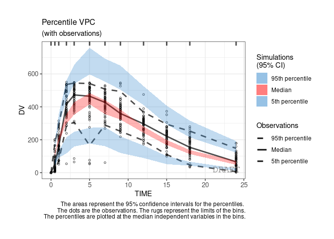
By default the vpc plot is percentile ; , but we can plot the scatter type:
ctr %>% pmx_plot_vpc(type ="scatter")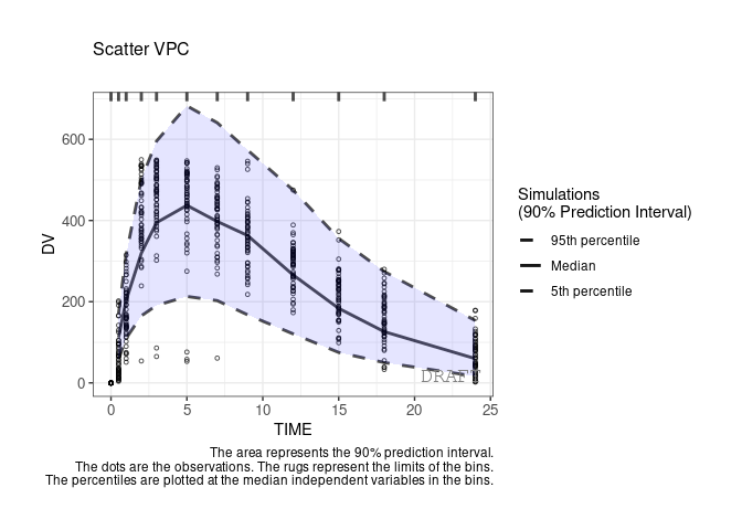
ctr %>% pmx_plot_vpc(bin=pmx_vpc_bin(style = "kmeans",n=5))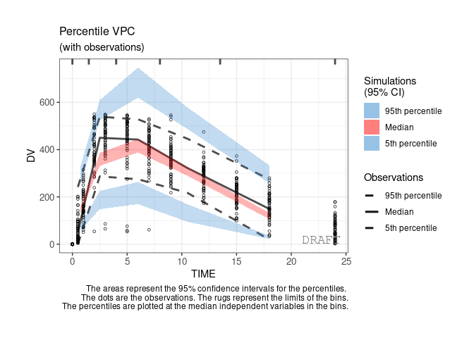
ctr %>% pmx_plot_vpc(labels = c(x = "DV axis", y = "TIME axis"))
ctr %>% pmx_plot_vpc(strat.facet=~SEX,facets=list(nrow=2))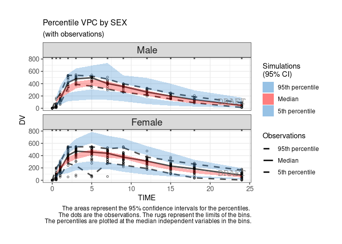
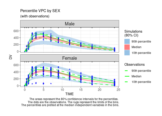
User can customize the options to get a Monolix-like display.
ctr %>% pmx_plot_vpc(
  strat.facet=~SEX,
  facets=list(nrow=2),
  type="percentile",
  is.draft = FALSE,
  pi = pmx_vpc_pi(interval = c(0.1,0.9),
              median=list(color="green"),
              extreme= list(color="green")),
  obs = pmx_vpc_obs(color="blue",shape=18,size=2),
  ci = pmx_vpc_ci(interval = c(0.1,0.9),
              median=list(fill="red"))
)
A report (in pdf and docx format) containing all default diagnostic plots can be created using the pmx_report function. The output can take three different values:
name.pdf and name.png specified in argument
name, located in save_dir) with default diagnostic
plotsggpmx_GOF by default, if parameter is not
specified) located in save_dir that contains all default
diagnostic plots, each in a pdf and png file. The different plots are
numerated in order to have an unique identifier for each plot (ex:
ebe_box-1.pdf). This is necessary for having correct footnotes that
indicated the path to the source file (for submission reports).Example:
ctr %>% pmx_report(name='Diagnostic_plots2',
                   save_dir = work_dir,
                   plots_subdir = "ggpmx_report",
                   output='all')
Note that running the same command first with the option “output=‘plots’” and then with the option “output=‘report’” will remove the ggpmx_GOF folder.
Note also that by default, the report will have the DRAFT label on all plots. The label can be removed by using the settings argument in the Controller creation.
The user can customize the default report by creating a “template”. To create a template, the user should create first a default report with the following command:
ctr %>% pmx_report(name='Diagnostic_plots1',
                   save_dir = work_dir,
                   plots_subdir = "ggpmx_report",
                   output='report')
The Rmarkdown (.Rmd) file is the “template”. The user can modify the Rmarkdown file as desired (ex: changing the size of some figures) and save the modified file. The new template can be used with the following command:
ctr %>% pmx_report(name='Diagnostic_plots3',
                   save_dir = work_dir,
                   plots_subdir = "ggpmx_report",
                   output='report',
template=file.path(work_dir,'Diagnostic_plots1.Rmd'))Any particular plot can be customized in two ways:
ctr %>% pmx_plot_xx(list of options)ctr %>% pmx_update(???xx???, list of options)Help(pmx_gpar) lists some options.
Help(pmx_plot_xx) lists some possible parameters to update a particular plot.
To obtain an exhaustive list of possible options for a particular plot, use the following:
ctr %>% get_plot_config("xx")It is possible to visualize BLQ (below the limit of quantification)
values in the individual plots. For this, bloq needs to be
specified using the pmx_bloq function (see example below with the
pmx_mlxtran() function).
ctr %>% pmx_mlxtran(file_name = mlx_file, bloq=pmx_bloq(cens = ???BLQ???, limit = ???LIMIT???))
ctr %>% pmx_plot_individual()Monolix users may want to plot simulated BLQs. This is possible for outputs with Monolix 2018 and later. An additional dataset is loaded (sim_blq), which will be used for plotting insted the regular “predictions”-dataset.
The sim_blq statment can be specified within the plot
(locally) …
ctr %>% pmx_mlxtran(file_name = mlx_file))
ctr %>% pmx_plot_iwres_ipred(sim_blq = TRUE)
… or within the controller (globally). If this statment is used within the controller, all corresponding plots will plot simulated BLOQs by default.
ctr %>% pmx_mlxtran(file_name = mlx_file, sim_blq = TRUE))
ctr %>% pmx_plot_iwres_ipred()pmx_settings()The user can define a Controller with global settings that will be applied to all plots. For example remove draft annoataion, use abbreviation defintions to define axis labels, etc.
A settings object is defined by using the function
pmx_settings(). The created object is passed as the
parameter “settings” to pmx(). By doing so, the settings
are defined globally and apply to all plots. For a complete list of
global settings with their corresponding default values, please consult
the ggPMX Help (?pmx_settings).
## set one or more settings
my_settings <- pmx_settings(
  is.draft   = FALSE,
  use.abbrev = TRUE,
  ...) ### set other settings parameters here
ctr <-
  pmx_mlx(
    ..., ## put here other pmx parametes
    settings = my_settings
) By default in the “standing” configuration, a DRAFT label is printed
on all plots. In order to switch this label off, the user sets the
is.draft option of pmx_settings() to
FALSE.
ctr <- theophylline(settings = pmx_settings(is.draft = FALSE))The order of factors in a facet plot is determined by the data contained in the predictions data frame. Ordering of facet panels can be performed by changing the factor specification for facet columns in the predictions data frame.
The example below defines a Controller with changed SEX facet panels order: 1 will be plotted before 0 rather than the other way round.
ctr <- theophylline()
ctr[["data"]][["predictions"]][["SEX"]] <-
  factor(ctr[["data"]][["predictions"]][["SEX"]], levels=c("1","0"))

pmx_plot_iwres_ipred(ctr, strat.facet=~SEX)The standing configuration initializes all plots using abbreviations for axis labels. Each abbreviation has its corresponding definition. To get the list of abbreviation :
ctr %>% get_abbrev
#> NULL
You can update one abbreviation to set a custom label
ctr %>% set_abbrev(TIME="TIME after the first dose")Using use.abbrev flag you can use abbreviation
definition to set axis labels:
ctr <- theophylline(settings=pmx_settings(use.abbrev = TRUE))
ctr %>% set_abbrev(TIME="Custom TIME axis")
ctr %>% pmx_plot_npde_time
finegrid.txt file for individual plotswithin Monolix, user can choose to not use finegrid file even if it is present.
ctr <- theophylline()
ctr %>% pmx_plot_individual(use.finegrid =FALSE, legend.position="top")
#> USE predictions data set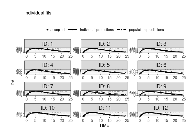
In case of color startfication user can customize the legend. For
example here using the ggplot2::scale_color_manual:
ctr <- theophylline()
ctr %>% pmx_plot_npde_time(strat.color="STUD")+
      ggplot2::scale_color_manual(
        "Study",
        labels=c("Study 1","Study 2"),
        values=c("1"="green","2"="blue"))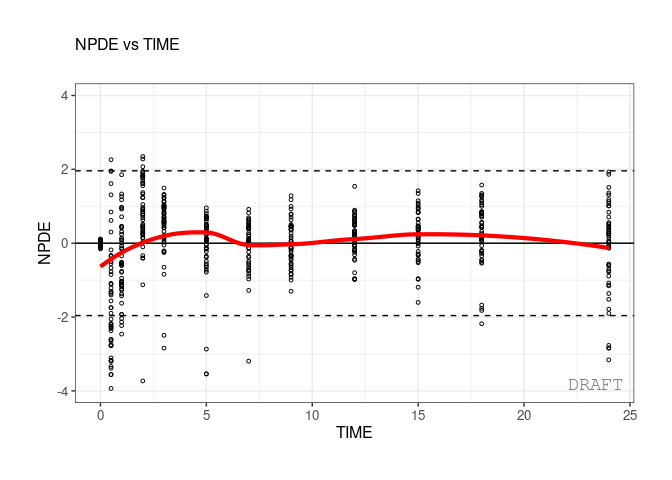
Another way to do it is to define a global scales.color
parameter that will applied to all plots with strat.color :
ctr <- theophylline(
  settings=
    pmx_settings(
      color.scales=list(
        "Study",
        labels=c("Study 1","Study 2"),
        values=c("1"="orange","2"="magenta"))
    )
)

ctr %>% pmx_plot_npde_time(strat.color="STUD")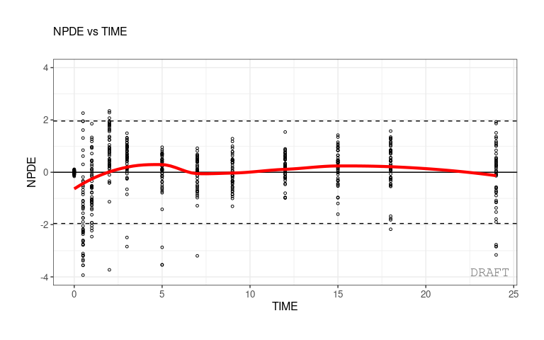
ctr %>% pmx_plot_eta_box(strat.color="STUD")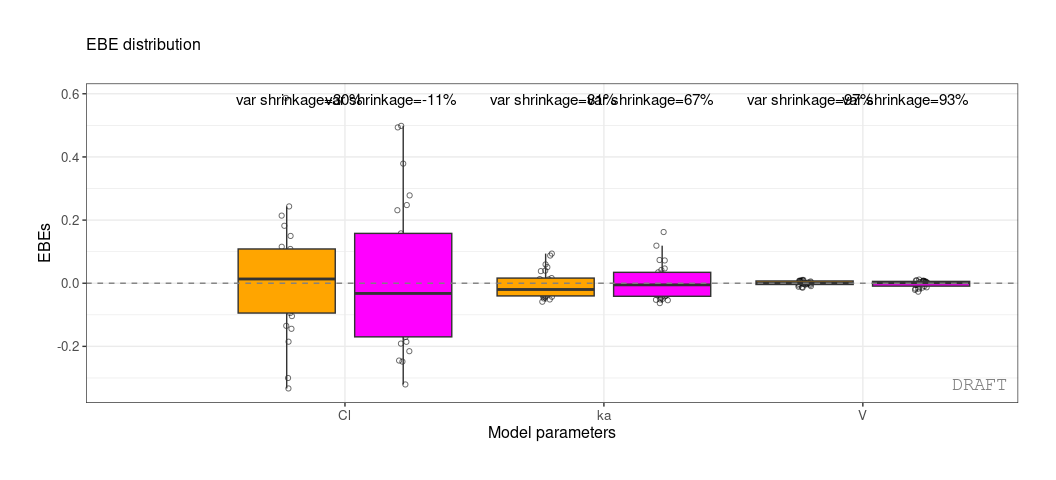
In case of faceting by stratification user can redfine categorical
labels to have more human readables strips. Lables are defined within
cats.labels argument and user can use them by setting
use.lables to TRUE.
ctr <- theophylline(
  settings=
    pmx_settings(
      cats.labels=list(
        SEX=c("0"="M","1"="F"),
        STUD=c("1"="Study 1","2"="Study 2")
      ),
      use.labels = TRUE
    )
)

ctr %>% pmx_plot_npde_time(strat.facet=~SEX)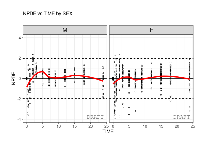
ctr <- theophylline(
  settings=
    pmx_settings(
      cats.labels=list(
        SEX=c("0"="M","1"="F"),
        STUD=c("1"="Study 1","2"="Study 2")
      ),
      use.labels = TRUE
    )
)

ctr %>% pmx_plot_npde_time(strat.facet=~SEX)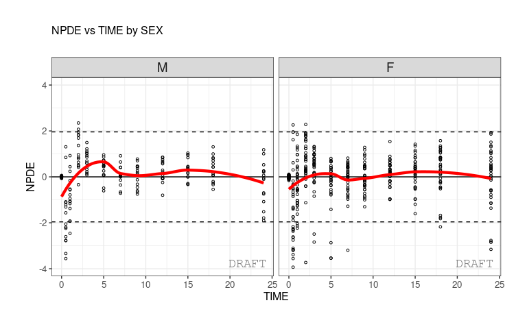
ctr %>% pmx_plot_eta_box(strat.facet =~SEX)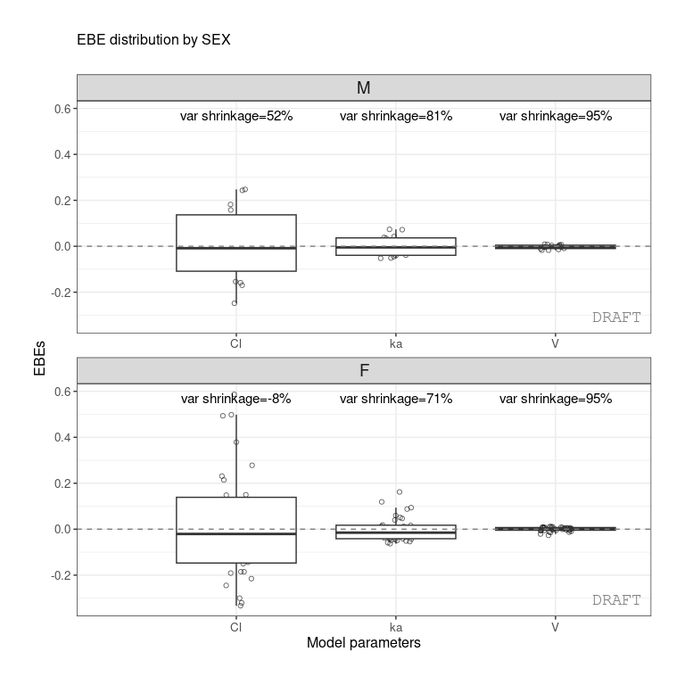
The type of binning used for VPC plots can be applied as an update to the controller object, causing the binning to be applied to subsequent VPC plots.
Updating the controller is achieved using pmx_update in
a command like:
pmx_update(ctr, "pmx_vpc", bin=pmx_vpc_bin(within_strat=TRUE, style="jenks"))Subsequent VPC plotting calls will then use “jenks” style binning. For example:
ctr %>% pmx_plot_vpcpmx()The function pmx() is the generic function for greating
a Controller. The user needs to specify a set of arguments such as the
path to the model directory, the software used for model fitting
(Monolix or nlmixr), the name of a configuration. A list of all existing
configurations is provided in the Appendix. All
mandatory arguments of pmx() are listed in
Table .
The example below defines a Controller with the standing (standard) configuration.
theophylline_path <- file.path(system.file(package = "ggPMX"), "testdata", "theophylline")
work_dir          <- file.path(theophylline_path, "Monolix")
input_data_path   <- file.path(theophylline_path, "data_pk.csv")

ctr <- pmx(
  sys       = "mlx",
  config    = "standing",
  directory = work_dir,
  input     = input_data_path,
  dv        = "Y",
  dvid      = "DVID"
)
Note that the column “DVID” of data_pk.csv does not exist; however it is not needed here because there is only one single output of the model. As dvid is a mandatory argument, it still needs to be provided and was set arbritrarly to “DVID” in the example above.
The input dataset can be provided to ggPMX via its location (as in
the example above) or as a data frame (maybe give an example). The
modeling output datasets have to be in the location that is indicated as
working directory (work_dir in the example above).
ggPMX is compatible with Monolix versions 2016 and later, NONMEM version 7.2 and later, and nlmixr.
In order to be able to produce all available diagnostic plots, the following tasks should be executed in Monolix during the model fitting procedure:
In addition, make sure to export charts data (In Monolix 2018: Settings -> Preferences -> Export -> switch on the Export charts data button). Select at least the following plots to be displayed and saved: individual fits and scatter plot of the residuals.
NONMEM Version 7.2/7.3/7.4 Preferred output tables according ???sdtab, patab, cotab, catab??? convention Simulation are required for creation of VPC (e.g. sdtab1sim)
Fit objects need to be generated by nlmixr and have data attached.
Standard errors are required (a successful covariance plot) for full
diagnostic checks. Can use boostrapFit() to get standard
error estimates if necessary
The main target of ggPMX is to create a report containing the following plots (see abbreviation list below):
Abbreviations:
ggPMX implements few functions to generate and
manipulate diagnostic plots. (Should we list pmx and pmx_mlx separately
and say the differences? Or it’s maybe clear from the previous
sections.)
(Apparently, it’s not the full list. Add all functions.) The design
of the package is around the central object: the controller. It can
introspected or piped using the %>% operand.
Note that:
The controller is an R6 object, it behaves like a
reference object. Some functions (methods) can have a side effect on the
controller and modify it internally. Technically speaking we talk about
chaining not piping here. However, using pmx_copy user can
work on a copy of the controller.
Graphical parameters in ggPMX are set internally using
the pmx_gpar function. A number of graphical parameters can
be set for the different plot types.
args(pmx_gpar)
#> function (is.title, labels, axis.title, which_pages, print, axis.text,
#>     ranges, is.smooth, smooth, is.band, band, is.draft, draft,
#>     discrete, is.identity_line, identity_line, smooth_with_bloq,
#>     scale_x_log10, scale_y_log10, color.scales, is.legend, legend.position)
#> NULL
More information can be found in the help document
?pmx_gpar and in the examples that follow.
For the moment we are mainly using standing configuration. In the next release user can specfiy configuration either by cretaing a custom yaml file or an R configuration object. Also ggPMX will create many helper functions to manipulate the configuration objects.
The shrinkage is a computation within controller data. In general it
is used to annotate the plots. Although one can get it independently
from any plot using pmx_comp_shrink. It is part of the
pmx_compt_xx layer( In the future we will add ,
pmx_comp_cor , pmx_comp_summary,..)
Here the basic call:
ctr %>% pmx_comp_shrink
#>    EFFECT   OMEGA    SHRINK       POS FUN
#> 1:     Cl 0.22485 0.1125175 0.2934250 var
#> 2:      V 0.03939 0.9469996 0.0057915 var
#> 3:     ka 0.10024 0.7423478 0.0810850 var
We get the shrinkage for each effect (SHRINK column).
The same values can be shown on distribution plot , for example :
ctr %>% pmx_plot_eta_box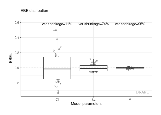 or :
or :
ctr %>% pmx_plot_eta_hist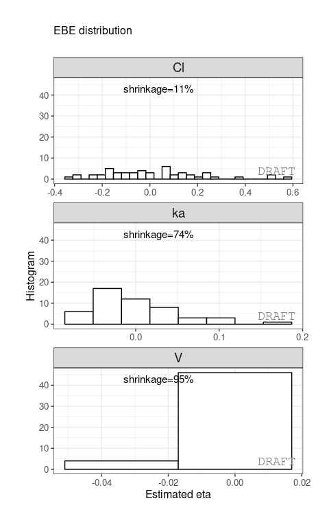
You can add or remove shrinkage annotation using
is.shrink argument ( TRUE by default) :
ctr %>% pmx_plot_eta_box( is.shrink = FALSE) 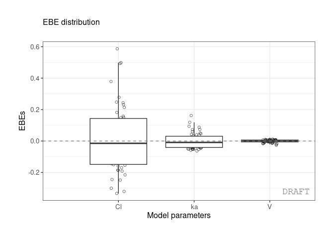
You can compute shrinkage by applying either standard deviation
sd or variance var :
ctr %>% pmx_comp_shrink(  fun = "var")
#>    EFFECT   OMEGA    SHRINK       POS FUN
#> 1:     Cl 0.22485 0.1125175 0.2934250 var
#> 2:      V 0.03939 0.9469996 0.0057915 var
#> 3:     ka 0.10024 0.7423478 0.0810850 var
ctr %>% pmx_plot_eta_box( shrink=pmx_shrink(fun = "var"))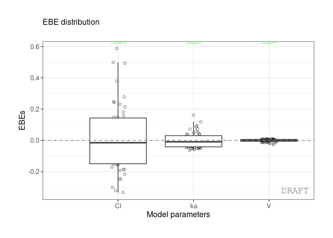
Note that for plotting functions which take a shrink parameter, this
can be created using the pmx_shrink function to create a
pmxShrinkClass object (or it can be a list which can be
converted into such an object using pmx_shrink).
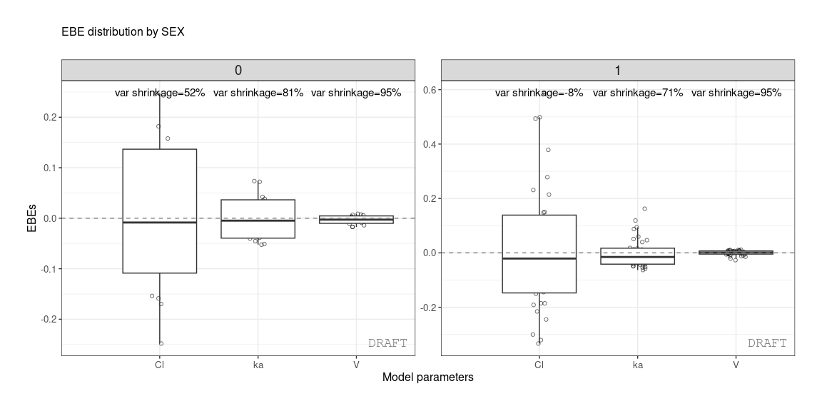
Shrinkage can be applied after stratification :
ctr %>% pmx_comp_shrink(strat.facet = ~SEX)
#>    EFFECT SEX   OMEGA      SHRINK        POS FUN
#> 1:     Cl   1 0.22485 -0.08032359 0.29342500 var
#> 2:     Cl   0 0.22485  0.51828810 0.12378000 var
#> 3:      V   1 0.03939  0.94628054 0.00579150 var
#> 4:      V   0 0.03939  0.94818243 0.00437235 var
#> 5:     ka   1 0.10024  0.70737008 0.08108500 var
#> 6:     ka   0 0.10024  0.80907530 0.03676950 var
or by grouping like :
ctr %>% pmx_comp_shrink(strat.color = "SEX")
#>    EFFECT SEX   OMEGA      SHRINK        POS FUN
#> 1:     Cl   1 0.22485 -0.08032359 0.29342500 var
#> 2:     Cl   0 0.22485  0.51828810 0.12378000 var
#> 3:      V   1 0.03939  0.94628054 0.00579150 var
#> 4:      V   0 0.03939  0.94818243 0.00437235 var
#> 5:     ka   1 0.10024  0.70737008 0.08108500 var
#> 6:     ka   0 0.10024  0.80907530 0.03676950 var
We can
ctr %>% pmx_plot_eta_hist(is.shrink = TRUE, strat.facet = ~SEX,
facets=list(scales="free_y"))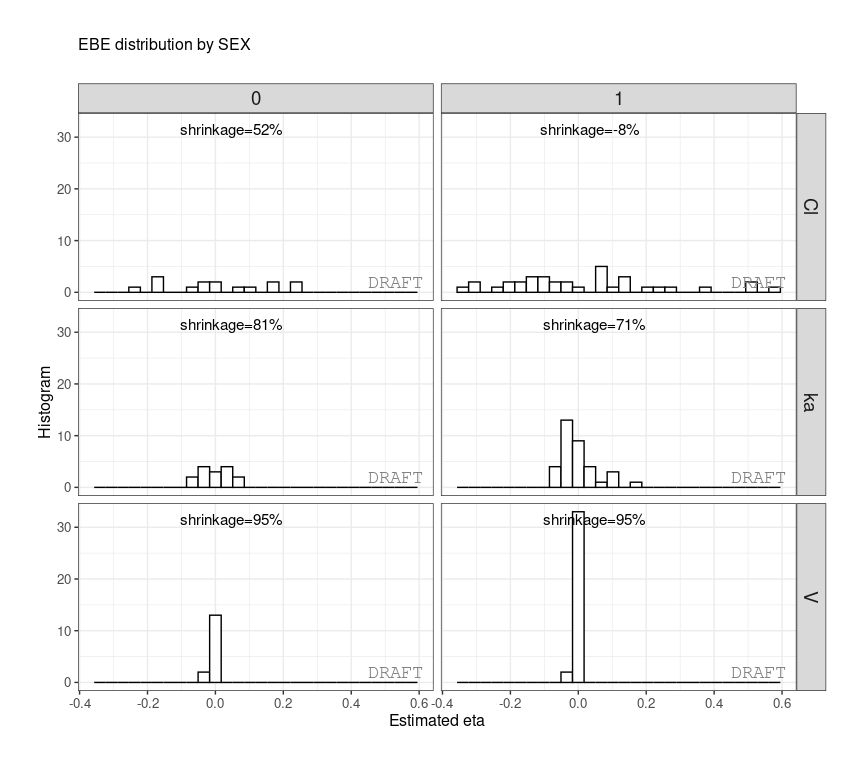 or
or
ctr %>% pmx_plot_eta_box(is.shrink = TRUE, strat.facet = "SEX",
                          facets=list(scales="free_y",ncol=2))