latexr

The goal of latexr is to translate LaTeX formulas to R code. (Formerly known as latex2r; the main function is still latex2r().)

Installation

You can install the development version from GitHub with:

# install.packages("devtools")
devtools::install_github("rodrigoesborges/latexr")

This is a very young package so it may not work as expected if you try to translate things outside of the supported syntax. Please refer to Supported LaTeX section for more information about it.

Examples

Just some basic functionality: translate LaTeX to R.

library(latexr)
latex2r("\\beta_1^{\\frac{x+1}{x^2 \\cdot y}}")
#> [1] "beta_1^((x + 1) / (x^2 * y))"

With a combination of parse() and eval() you can evaluate the translated expression. Of course, names must be bound to a value if we expect this to work.

eval(parse(text = latex2r("\\pi * \\sin(\\frac{x}{2})")), envir = list(x = pi))
#> [1] 3.141593

There is an extra feature which is possible due to R is so permissive. latex2fun() receives a LaTeX expression that represents the definition of a mathematical function and returns an R function that computes the function value and has arguments representing all the variables involved in the function.

x = seq(-2*pi, 2*pi, length.out = 500)
f = latex2fun("\\sin{a * x}^2 + \\cos{b * x} ^2")
print(f)
#> function (a, b, x) 
#> sin(a * x)^2 + cos(b * x)^2

y = f(x = x, a = 2, b = 3)
plot(x, y, type = "l")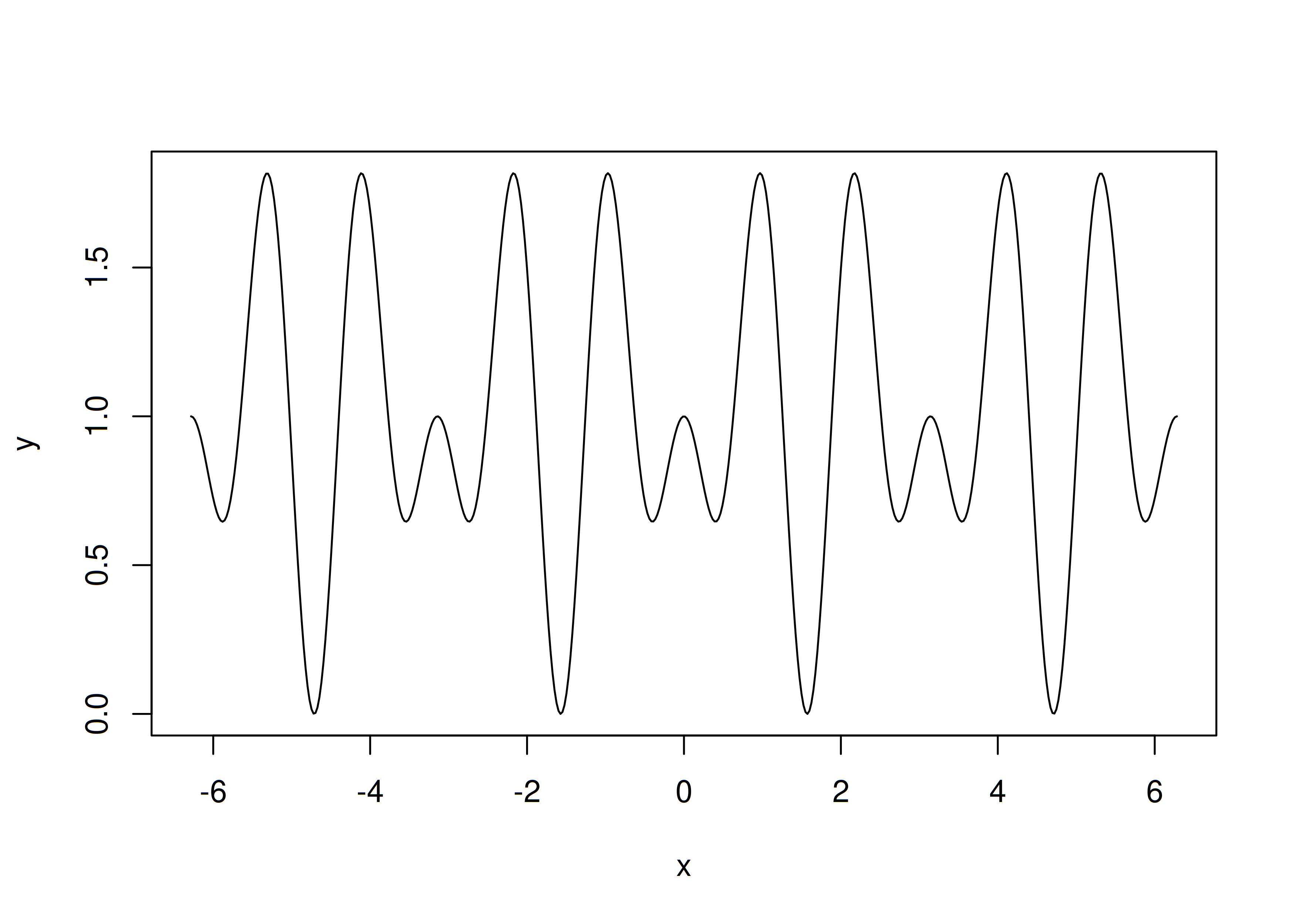

This is experimental but I think it is so cool that it is worth a chance in the package. For those who like to play with R most weird features, they would find the source code is a nice place.

In addition, if you call latex2r(interactive=TRUE) it launches a REPL that you can use interactively.

Supported LaTeX

Only a small subset of LaTeX expressions are supported so far. However, these are enough to define a very wide set of mathematical functions.

Greek letters supported

The following Greek letters are supported as identifiers (variable names).

latexr:::get_pkg_data('GREEK_KEYWORDS')
#>  [1] "\\alpha"      "\\theta"      "\\tau"        "\\beta"       "\\vartheta"  
#>  [6] "\\pi"         "\\upsilon"    "\\gamma"      "\\varpi"      "\\phi"       
#> [11] "\\delta"      "\\kappa"      "\\rho"        "\\varphi"     "\\epsilon"   
#> [16] "\\lambda"     "\\varrho"     "\\chi"        "\\varepsilon" "\\mu"        
#> [21] "\\sigma"      "\\psi"        "\\zeta"       "\\nu"         "\\varsigma"  
#> [26] "\\omega"      "\\eta"        "\\xi"         "\\Gamma"      "\\Lambda"    
#> [31] "\\Sigma"      "\\Psi"        "\\Delta"      "\\Xi"         "\\Upsilon"   
#> [36] "\\Omega"      "\\Theta"      "\\Pi"         "\\Phi"

Syntax supported

You can use the following operators

Unary:
- + and -.
Binary:
- +, -, *, /, ^, and _.
Grouping:
- {...}, \left{...\right}, (...), and \left(...\right).
Absolute value:
- \left|x\right|.

And the following functions

Unary:
- \sqrt, \log, \ln, \sin, \cos, \tan, \cosh, \sinh, and \tanh.
- Statistical: \bar{x} and \overline{x} (mean), and \tilde{x} (median).
Binary:
- \frac{...}{...}, \cdot, and \times.
- Rolling sum: \sum_{k}^{}{x} translates to data.table::frollsum(x, k).

Spacing commands (\;, \,, \:, \quad, \qquad) are ignored.

Notes

The operator _ is used to represent subscripts. While you can do $5_2$ in LaTeX, it is not allowed in the package since a subscript on a number does not make sense.
Only variable names (such as x or \\pi) can have subscripts.
In latex you can write \sqrt[p]{x} to represent the p-th root. However this is not allowed in this package (at least for now). To represent a p-th root you can use x^{1/p}.

Some remarks

Implicit multiplication

tl;dr: xy is understood as x times y.

A previous version of this package required multiplication to be explicit. For example, xy would have been understood as an identifier called xy. Now, all identifiers, except from special ones (Greek letters), are of one character only. If you do abc^5 it will be understood as a*b*c^5.

In addition, you can still pass an explicit multiplication operator such as *, \times or \cdot.

Explicit grouping

Although something like \sin5 renders as $\sin5$ and we all understand this means sine of 5, we require explicit grouping with {} or () to avoid ambiguity in the function argument. What if I write \sin5a? Does it mean a times the sine of 5 or the sine of 5 times a? Explicit grouping is a simple solution to eliminate this ambiguity.

Special treatment for some characters

Since the numbers $\pi$ and $e$ are so common in mathematical expressions they are treated as constant numbers and not as names of variables.

In R $\pi$ is a built-in constant number and $e$ is obtained with exp(1). See the next example

latex2r("\\sin{2 * \\pi * t}")
#> [1] "sin(2 * pi * t)"
latex2r("e * x")
#> [1] "exp(1) * x"
latex2r("e^{x + i * y}")
#> [1] "exp(x + i * y)"

But note that complex numbers are not supported (yet?).

Logarithm of different base

If you write \\log(x) it will be interpreted as the natural logarithm of x. If you write \\log_n(x) it will be interpreted as the logarithm of x with base n. The alias \\ln(x) also works.

latex2r("\\log(x + 1)")
#> [1] "log(x + 1)"
latex2r("\\log_2(x + 1)")
#> [1] "log(x + 1, base = 2)"
latex2r("\\ln(x + 1)")
#> [1] "log(x + 1)"

Statistical notation

\\bar{x} and \\overline{x} translate to mean(x), and \\tilde{x} translates to median(x). Since real data often contains missing values, both accept na.rm = TRUE:

latex2r("\\bar{x} + \\tilde{y}")
#> [1] "mean(x) + median(y)"
latex2r("\\bar{x} + \\tilde{y}", na.rm = TRUE)
#> [1] "mean(x, na.rm = TRUE) + median(y, na.rm = TRUE)"

For windowed calculations, \\sum_{k}^{}{x} translates to data.table::frollsum(x, k), a rolling sum of window k.

latex2r("\\sum_{3}^{}{x}")
#> [1] "data.table::frollsum(((x)), 3)"

Unicode input (MathQuill and friends)

Visual formula editors such as MathQuill emit raw Unicode characters instead of LaTeX commands. latex2r() normalizes them automatically before scanning: −, – and — become -; × becomes \times; ⋅ and · become \cdot; ÷ becomes /; Greek letters become the corresponding commands; and accented vowels such as ā, ã and â become \bar{a}, \tilde{a} and \hat{a} (other accents fall back to the base letter).

latex2r("2 × 3")
#> [1] "2 * 3"
latex2r("α + β")
#> [1] "alpha + beta"
normalize_mathquill("ā")
#> [1] "\\bar{a}"

The normalize_mathquill() function is exported so the mapping can be inspected and reused.

Inspecting the parsed expression

latex2ast() runs the same pipeline as latex2r() but returns the parsed abstract syntax tree instead of the R translation, which is useful for debugging formulas.

latex2ast("\\bar{x}")
#> <UnaryFun>
#>   Inherits from: <Expr>
#>   Public:
#>     accept: function (visitor) 
#>     arg: Variable, Expr, R6
#>     clone: function (deep = FALSE) 
#>     initialize: function (operator, arg) 
#>     operator: mean

Examples

LaTeX	R Code
`x + y`	`x + y`
`\sin(x) + \cos(y)`	`sin(x) + cos(y)`
`\sin(x)^2 + \cos(y)^2`	`sin(x)^2 + cos(y)^2`
`\sqrt{2x\pi}`	`sqrt(2 * x * pi)`
`\log(z)`	`log(z)`
`\ln(z)`	`log(z)`
`\log_a(\frac{x^5}{y})`	`log((x^5) / y, base = a)`
`\frac{1}{\sigma\sqrt{2\pi}}e^{\frac{(x - \mu)^2}{2\sigma^2}}`	`1 / (sigma * sqrt(2 * pi)) * exp(((x - mu)^2) / (2 * sigma^2))`
`\beta_1^{\frac{x+1}{x^2 \cdot y}}`	`beta_1^((x + 1) / (x^2 * y))`
`\bar{x}`	`mean(x)`
`\tilde{x}`	`median(x)`
`\left\|x + y\right\|`	`abs(x + y)`
`\sum_{3}^{}{x}`	`data.table::frollsum(x, 3)`