The goal of memoria is to provide the tools to quantify ecological memory in long time-series involving environmental drivers and biotic responses, including palaeoecological datasets.
Ecological memory has two main components: the endogenous component, which represents the effect of antecedent values of the response on itself, and endogenous component, which represents the effect of antecedent values of the driver or drivers on the current state of the biotic response. Additionally, the concurrent effect, which represents the synchronic effect of the environmental drivers over the response is measured. The functions in the package allow the user
The package memoria uses the fast implementation of Random Forest available in the ranger package to fit a model of the form shown in Equation 1:
Equation 1 (simplified from the one in the paper): [p_{t} = p_{t-1} +…+ p_{t-n} + d_{t} + d_{t-1} +…+ d_{t-n}]
Where:
Random Forest returns an importance score for each model term, and the functions in memoria let the user to plot the importance scores across time lags for each ecological memory components, and to compute different features of each memory component (length, strength, and dominance).
You can install the released version of memoria from GitHub or soon from CRAN with:
#from GitHub
library(devtools)
install_github("blasbenito/memoria")

#from CRAN (not yet)
install.packages("memoria")library(memoria)
#other useful libraries
library(ggplot2)
library(cowplot)
library(viridis)
library(tidyr)
library(kableExtra)To work with the memoria package the user has to provide a long time-series with at least one environmental driver and one biotic response. The steps below assume that the driver and the biotic response were taken at different temporal resolutions or depth intervals, but if that is not the case, the actual workflow would start at point 2.
1. Prepare data. The function mergePalaeoData allows the user to: 1) merge together environmental proxies/variables and biotic responses sampled at different time resolutions; 2) reinterpolate the data into a regular time grid using loess.
In this scenario we consider two datasets:
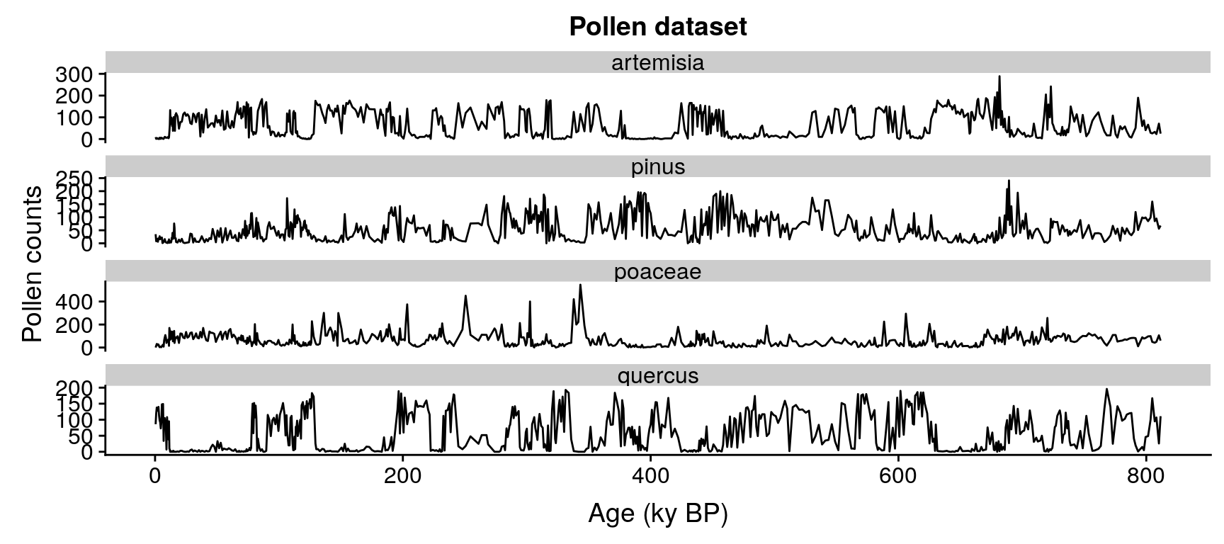
pollen, with 639 samples dated in ky BP and four pollen types: Pinus, Quercus, Poaceae, and Artemisia.
climate, with 800 samples dated in ky BP, and five climate variables: average temperature and rainfall, temperature of the warmest and coldest month, and oxigen isotope.
#loading and plotting pollen data
data(pollen)

#plotting the data
ggplot(data=gather(pollen, pollen.type, pollen.abundance, 2:5),
       aes(x=age,
           y=pollen.abundance,
           group=pollen.type)) +
  geom_line() +
  facet_wrap("pollen.type", ncol=1, scales = "free_y") +
  xlab("Age (ky BP)") +
  ylab("Pollen counts") +
  ggtitle("Pollen dataset")
#loading and plotting climate data
data(climate)

#plotting the data
ggplot(data=gather(climate, variable, value, 2:5),
       aes(x=age,
           y=value,
           group=variable)) +
  geom_line() +
  facet_wrap("variable", ncol=1, scales = "free_y") +
  xlab("Age (ky BP)") +
  ylab("") +
  ggtitle("Palaeoclimatic data")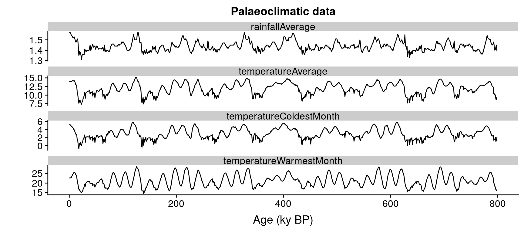
The datasets are not aligned, and pollen is not sampled at regular times, which makes any kind of analysis challenging. The code below fixes these issues by merging the data into the same regular time grid through the function mergePalaeoData. The function warns the user when the interpolation factor (difference between the original temporal resolution of the data and the interpolated resolution) is higher than one order of magnitude. Please, check the help file of the function to better understand how it works.
#merging and interpolating into a
#regular time grid of 0.2 ky resolution
pollen.climate <- mergePalaeoData(
 datasets.list = list(
   pollen=pollen,
   climate=climate
 ),
 time.column = "age",
 interpolation.interval = 0.2
 )
#> Argument interpolation.interval is set to 0.2
#> The average temporal resolution of pollen is 1.27; you are incrementing data resolution by a factor of 6.35
#> The average temporal resolution of climate is 1; you are incrementing data resolution by a factor of 5

str(pollen.climate)
#> 'data.frame':    3993 obs. of  10 variables:
#>  $ age                            : num  0.5 0.7 0.9 1.1 1.3 1.5 1.7 1.9 2.1 2.3 ...
#>  $ pollen.pinus                   : num  0 2.5 6.97 10.64 13.39 ...
#>  $ pollen.quercus                 : num  95.6 109.4 120.1 127.7 132.6 ...
#>  $ pollen.poaceae                 : num  0 9.55 16.79 21.76 24.76 ...
#>  $ pollen.artemisia               : num  0 0 0.672 1.696 2.516 ...
#>  $ climate.temperatureAverage     : num  14.1 14.1 14 14 14 ...
#>  $ climate.rainfallAverage        : num  1.57 1.57 1.57 1.57 1.57 ...
#>  $ climate.temperatureWarmestMonth: num  21 21.3 21.5 21.7 21.8 ...
#>  $ climate.temperatureColdestMonth: num  5.25 5.24 5.23 5.22 5.2 ...
#>  $ climate.oxigenIsotope          : num  3.43 3.43 3.43 3.44 3.44 ...

#plotting the data
ggplot(data=gather(pollen.climate, variable, value, 2:10),
       aes(x=age,
           y=value,
           group=variable)) +
  geom_line() +
  facet_wrap("variable", ncol=1, scales = "free_y") +
  xlab("Age (ky BP)") +
  ylab("") +
  ggtitle("Pollen and palaeoclimate")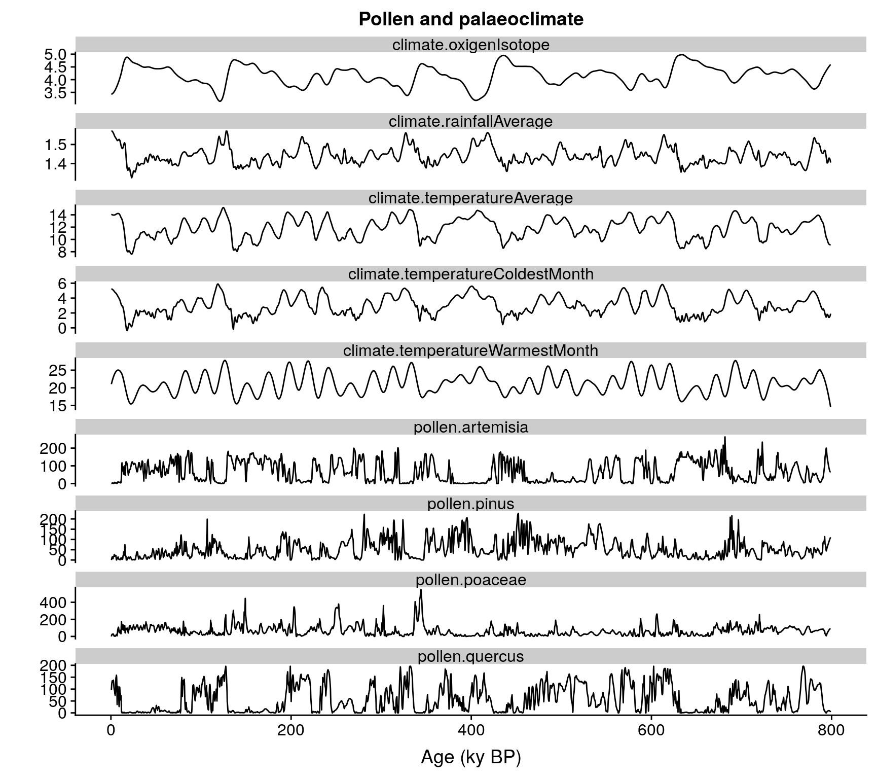
2. Organize the data in time lags. To fit the model in Equation 1 it is required to select a response variable, a set of drivers (or a single driver), and organize the data in lags, so every sample in the response column is aligned with antecedent values of the response and the environmental drivers for a given set of lags. The function prepareLaggedData generates a dataframe with one column per term in Equation 1. In this case, we use the pollen abundance of Pinus as response varaible, and average temperature and rainfall as drivers/predictors.
pollen.climate.lagged <- prepareLaggedData(
 input.data = pollen.climate,
 response = "pollen.pinus",
 drivers = c("climate.temperatureAverage", "climate.rainfallAverage"),
 time = "age",
 oldest.sample = "last",
 lags = seq(0.2, 1, by=0.2),
 time.zoom=NULL,
 scale=FALSE
)
str(pollen.climate.lagged)
#> 'data.frame':    3988 obs. of  19 variables:
#>  $ Response_0                    : num  0 2.5 6.97 10.64 13.39 ...
#>  $ Response_0.2                  : num  2.5 6.97 10.64 13.39 15.02 ...
#>  $ Response_0.4                  : num  6.97 10.64 13.39 15.02 15.62 ...
#>  $ Response_0.6                  : num  10.6 13.4 15 15.6 14.5 ...
#>  $ Response_0.8                  : num  13.4 15 15.6 14.5 10.9 ...
#>  $ Response_1                    : num  15 15.6 14.5 10.9 6 ...
#>  $ climate.temperatureAverage_0  : num  14.1 14.1 14 14 14 ...
#>  $ climate.temperatureAverage_0.2: num  14.1 14 14 14 14 ...
#>  $ climate.temperatureAverage_0.4: num  14 14 14 14 14 ...
#>  $ climate.temperatureAverage_0.6: num  14 14 14 14 14 ...
#>  $ climate.temperatureAverage_0.8: num  14 14 14 14 14 ...
#>  $ climate.temperatureAverage_1  : num  14 14 14 14 14 ...
#>  $ climate.rainfallAverage_0     : num  1.57 1.57 1.57 1.57 1.57 ...
#>  $ climate.rainfallAverage_0.2   : num  1.57 1.57 1.57 1.57 1.57 ...
#>  $ climate.rainfallAverage_0.4   : num  1.57 1.57 1.57 1.57 1.57 ...
#>  $ climate.rainfallAverage_0.6   : num  1.57 1.57 1.57 1.57 1.57 ...
#>  $ climate.rainfallAverage_0.8   : num  1.57 1.57 1.57 1.57 1.56 ...
#>  $ climate.rainfallAverage_1     : num  1.57 1.57 1.57 1.56 1.56 ...
#>  $ time                          : num  0.5 0.7 0.9 1.1 1.3 1.5 1.7 1.9 2.1 2.3 ...
Extra attention should be paid to the oldest.sample argument. When it is set to “last”, as above, it assumes that the dataframe is ordered (top to bottom) by depth/age, and therefore represents a palaeoecological dataset. In this case, the lag 1 of the first sample is the second sample. If it is set to “first”, it assumes that the first sample defines the beginning of the time series. In such a case, the lag 1 of the second sample is the first sample.
Also note that: * The resoponse column is identified with the string Response_0 (as in “value of the response for the lag 0”). * The endogenous memory terms are identified with the pattern Response[0.2 - 1], with the numbers indicating the lag (in the same units as the time column). * The exogenous memory terms are identified by the name of the climatic variables followed by the lags between 0.2 and 1. * The concurrent effect is identified by the names of the climate variables with the lag 0.
3. Fit Random Forest model on the lagged data to assess ecological memory. The function computeMemory fits a Random Forest on the lagged data following Equation 1. It does so by using the implementation of Random Forest available in the ranger package. This is the fastest Random Forest implementation available to date, and has the ability to use every processor available in a computer, considerably speeding up the model-fitting process.
The goal of computeMemory is to measure the importance of every term in Equation 1. Random Forest provides a robust measure of variable importance that is insensitive to multicollinearity or temporal autocorrelation in the input dataset. It is based on the loss of accuracy when a given predictor is randomly permuted across a large number of regression trees (please, see the vignette for further information).
However, Random Forest does not provide any measure of significance, making it difficult to assess when the importance of a given predictor is the result of chance. To solve this issue, computeMemory adds a new term, named r, to Equation 1. This new term is either a totally random sequence of numbers (mode white.noise) or a time series with a temporal autocorrelation generated randomly (mode autocorrelated). Both serve as a sort of null test, but using the autocorrelated mode provides much more robust results.
The model is then repeated a number of times defined by the user (check the repetitions argument in the help of the computeMemory function), the r term is generated again with a different random seed on each repetition, and after all iterations have been performed, the percentiles 0.05, 0.5, and 0.95 of the importance of each equation term are computed and provided in the output dataframe.
The output can be easily plotted with the plotMemory function. The example below is done with a low number of repetitions to reduce runtime, but note that the recommended number of iterations should be higher (300 gives stable results for time series with around 500 samples).
#computing memory
memory.output <- computeMemory(
 lagged.data = pollen.climate.lagged,
 drivers = c("climate.temperatureAverage",
             "climate.rainfallAverage"),
 response = "Response",
 add.random = TRUE,
 random.mode = "white.noise",
 repetitions = 100
)

#the output is a list with 4 slots

#the memory dataframe
head(memory.output$memory)
#>                                median        sd      min      max
#> Response_0.2                 63.72511 0.7163610 62.51069 64.80383
#> Response_0.4                 51.16831 0.7463974 50.01752 52.44615
#> Response_0.6                 40.96195 0.6979277 39.82137 41.95080
#> Response_0.8                 35.68578 1.1570548 33.91781 37.52504
#> Response_1                   42.84917 0.9537612 41.14918 44.09713
#> climate.temperatureAverage_0 41.88860 3.4182192 34.03551 45.14606
#>                                                Variable Lag
#> Response_0.2                                   Response 0.2
#> Response_0.4                                   Response 0.4
#> Response_0.6                                   Response 0.6
#> Response_0.8                                   Response 0.8
#> Response_1                                     Response 1.0
#> climate.temperatureAverage_0 climate.temperatureAverage 0.0

#predicted values
head(memory.output$prediction)
#>       median         sd       min       max
#> X1  4.855762 0.13624378  4.603849  5.050147
#> X2  5.588746 0.12595703  5.411583  5.831361
#> X3  7.616612 0.12654352  7.407159  7.799427
#> X4 11.107384 0.14786080 10.908995 11.413256
#> X5 13.472921 0.11391455 13.313259 13.666736
#> X6 14.252521 0.09672598 14.105857 14.398320

#pseudo R-squared of the predictions
head(memory.output$R2)
#> [1] 0.9877769 0.9877619 0.9875986 0.9876862 0.9877391 0.9878348

#VIF test on the input data
#VIF > 5 indicates significant multicollinearity
head(memory.output$multicollinearity)
#>                       variable         vif
#> 1                 Response_0.2    27.46575
#> 2                 Response_0.4    74.98629
#> 3                 Response_0.6    77.78521
#> 4                 Response_0.8    75.03215
#> 5                   Response_1    27.42287
#> 6 climate.temperatureAverage_0 15232.75139

#plotting the memory pattern
plotMemory(memory.output) are represented by blue and green, and the random component is represented in yellow. The lag 0 of rainfall and precipitation represents the concurrent effect.")
Below the model is repeated by using “auatocorrelated” in the argument random.mode.
#computing memory
memory.output.autocor <- computeMemory(
 lagged.data = pollen.climate.lagged,
 drivers = c("climate.temperatureAverage",
             "climate.rainfallAverage"),
 response = "Response",
 add.random = TRUE,
 random.mode = "autocorrelated",
 repetitions = 100
)

#plotting the memory pattern
plotMemory(memory.output.autocor)
Finally, the features of the ecological memory pattern can be extracted. These features are:
memory strength: Maximum difference in relative importance between each component (endogenous, exogenous, and concurrent) and the median of the random component. This is computed for exogenous, endogenous, and concurrent effect.
memory length: Proportion of lags over which the importance of a memory component is above the median of the random component. This is only computed for endogenous and exogenous memory.
dominance: Proportion of the lags above the median of the random term over which a memory component has a higher importance than the other component. This is only computed for endogenous and exogenous memory.
memory.features <- extractMemoryFeatures(
  memory.pattern = memory.output.autocor,
  exogenous.component = c(
  "climate.temperatureAverage",
  "climate.rainfallAverage"
  ),
  endogenous.component = "Response",
  sampling.subset = NULL,
  scale.strength = TRUE
  )

kable(memory.features)|
label |
strength.endogenous |
strength.exogenous |
strength.concurrent |
length.endogenous |
length.exogenous |
dominance.endogenous |
dominance.exogenous |
|---|---|---|---|---|---|---|---|
|
1 |
1 |
NaN |
1 |
0.4 |
0 |
0.4 |
0 |