When unidentified human remains are found, forensic scientists must search databases of missing persons to find potential identifications. mispitools provides a statistical framework based on likelihood ratios (LRs) to quantify the weight of evidence, combining genetic and non-genetic information, and support decision-making in these investigations.
The likelihood ratio is the gold standard for evidence evaluation in forensic science. Rather than providing a binary “yes/no” answer, the LR tells us how much the evidence should change our belief about an identification.
We evaluate evidence under two competing hypotheses:
\[LR = \frac{P(\text{Evidence} \mid H_1)}{P(\text{Evidence} \mid H_2)}\]
The LR is not a probability of identification. It measures the relative support provided by the evidence, which can then be combined with prior information to make decisions.
# From CRAN
install.packages("mispitools")

# Development version
devtools::install_github("MarsicoFL/mispitools")Consider a realistic scenario: a family reports a person missing, and investigators need to search a database of unidentified individuals. The family provides a DNA sample from a relative (e.g., a grandparent), and investigators have information about the missing person’s physical characteristics.
We simulate LR distributions from DNA evidence. This requires defining a pedigree structure connecting the MP to the reference individual who provided a DNA sample.
library(mispitools)
library(forrel)
library(pedtools)

# Define pedigree: grandparent-grandchild relationship
ped <- linearPed(2)  # 3-generation pedigree
ped <- setMarkers(ped, locusAttributes = NorwegianFrequencies[1:15])
ped <- profileSim(ped, N = 1, ids = 2)  # Simulate reference profile

# Simulate LRs under both hypotheses
lr_dna <- sim_lr_genetic(ped, missing = 5, numsims = 500)
lr_dna_df <- lr_to_dataframe(lr_dna)

head(lr_dna_df)
#>      Related  Unrelated
#> 1  1247.3201  0.0023415
#> 2   892.1547  0.0001823
#> ...
The Related column contains LRs simulated under H1 (when
the POI truly is the MP), while Unrelated contains LRs
under H2 (when the POI is unrelated).
Physical characteristics such as biological sex, estimated age, and anthropological features also provide evidential value:
# Simulate LR distributions for sex and age
lr_sex <- sim_lr_prelim("sex", numsims = 500)
lr_age <- sim_lr_prelim("age", numsims = 500)

head(lr_sex)
#>    Related Unrelated
#> 1    1.863    0.1052
#> 2    1.863    1.8627
#> ...When evidence sources are conditionally independent, their LRs multiply. This is a fundamental property of the Bayesian framework:
# Combine DNA + sex + age
lr_total <- lr_combine(lr_dna_df, lr_sex)
lr_total <- lr_combine(lr_total, lr_age)

# Visualize the combined LR distribution
plot_lr_distribution(lr_total)
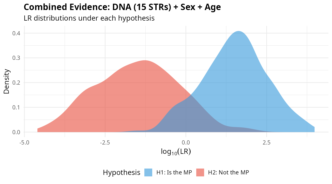
The separation between distributions under H1 (blue) and H2 (red) reflects the discriminating power of the combined evidence. Greater separation means better ability to distinguish between the two hypotheses.
In practice, we search databases containing unidentified individuals. Each candidate receives an LR based on all available evidence, and candidates are ranked accordingly:
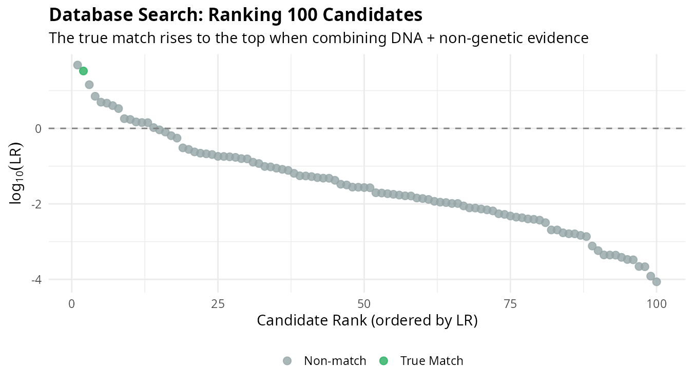
The individual corresponding to the actual MP (blue) rises to the top of the ranking. This demonstrates how combining multiple evidence sources improves our ability to identify the correct individual among many candidates.
To convert LRs into decisions, we analyze error rates at different thresholds:
# Find optimal threshold balancing false positives and false negatives
threshold <- decision_threshold(lr_total, weight = 10)

# Examine error rates at this threshold
threshold_rates(lr_total, threshold)
The weight parameter reflects the relative cost of false
positives versus false negatives. In forensic contexts, falsely
identifying someone (false positive) is typically considered more
serious than failing to identify (false negative).
For users who prefer a graphical interface, mispitools includes an interactive Shiny application:
mispitools_app()The app is also available online at: https://francomarsico.shinyapps.io/mispitools/
It provides tools for calculating LRs from non-genetic evidence, visualizing probability tables, and exploring decision thresholds.
| Function | Purpose |
|---|---|
sim_lr_genetic() |
Simulate LRs from DNA evidence |
sim_lr_prelim() |
Simulate LRs from non-genetic evidence |
lr_combine() |
Combine independent evidence sources |
lr_to_dataframe() |
Convert genetic LR results to data frame |
decision_threshold() |
Find optimal classification threshold |
threshold_rates() |
Compute error rates at a given threshold |
plot_lr_distribution() |
Visualize LR distributions |
mispitools_app() |
Interactive Shiny application |
Marsico FL, Caridi I (2023). “Incorporating non-genetic evidence in large scale missing person searches: A general approach beyond filtering.” Forensic Science International: Genetics, 66, 102891. https://doi.org/10.1016/j.fsigen.2023.102891
Marsico FL, Vigeland MD, et al. (2021). “Making decisions in missing person identification cases with low statistical power.” Forensic Science International: Genetics, 52, 102519. https://doi.org/10.1016/j.fsigen.2021.102519
Egeland T, Marsico FL (2026). “Using all available information in missing person identification.” Under review.
Franco L. Marsico — Creator and Head Maintainer
Main contributors: - Suisei Nakagawa - Undral Ganbaatar
GPL-3