
Extending mlr3 to time series forecasting.




This package is in an early stage of development and should be considered experimental. If you are interested in experimenting with it, we welcome your feedback!
Install the last release from CRAN:
install.packages("mlr3forecast")Install the development version from GitHub:
# install.packages("pak")
pak::pak("mlr-org/mlr3forecast")mlr3forecast extends the mlr3 ecosystem to time series forecasting. It introduces a forecasting task, forecasting learners, temporal resampling strategies, forecasting measures, and feature-engineering pipe operators, so that forecasters behave like any other mlr3 learner — ready for tuning, benchmarking, pipelines, and ensembling.
At a glance, mlr3forecast provides:
Classical forecasters wrapping forecast, smooth,
prophet, and tscount — over 30 in total, from baselines
(fcst.mean, fcst.random_walk) to ARIMA
(fcst.auto_arima), ETS, theta, TBATS, prophet, neural nets
(fcst.nnetar), and count models
(fcst.tscount). See mlr_learners$keys("^fcst")
for the full list.
Machine learning forecasting that turns any
regr learner into a forecaster via lag features, with both
recursive (one model applied iteratively) and
direct (one model per horizon) strategies.
Forecasting tasks and temporal resamplings
(fcst.holdout, fcst.cv) that respect the order
of observations, plus global (longitudinal) forecasting across many
series.
Feature-engineering pipe operators such as
fcst.lags, fcst.rolling,
fcst.fourier, fcst.feasts, and
fcst.tsfeats.
Forecasting measures including MASE, RMSSE,
Pinball, Winkler, coverage, and MSIS (see
mlr_measures$keys("^fcst") for the full list).
Full mlr3 integration: tuning with mlr3tuning, benchmarking, target transformations, and ensembling with mlr3pipelines.
Example tasks to get started —
airpassengers, electricity,
livestock, lynx, and usaccdeaths.
List them with
as.data.table(mlr_tasks)[task_type == "fcst"].
For now the forecasting task and learner are restricted to time series regression, but may be extended to classification in the future.
Jump to the examples for:
Native forecasting learners are provided by packages such as forecast, smooth, prophet, and tscount.
library(mlr3forecast)
library(mlr3pipelines)
library(ggplot2)

task = tsk("airpassengers")
task
#>
#> ── <TaskFcst> (144x1): Monthly Airline Passenger Numbers 1949-1960 ─────────────
#> • Target: passengers
#> • Properties: ordered
#> • Order by: month
#> • Frequency: month

# or plot the task
autoplot(task)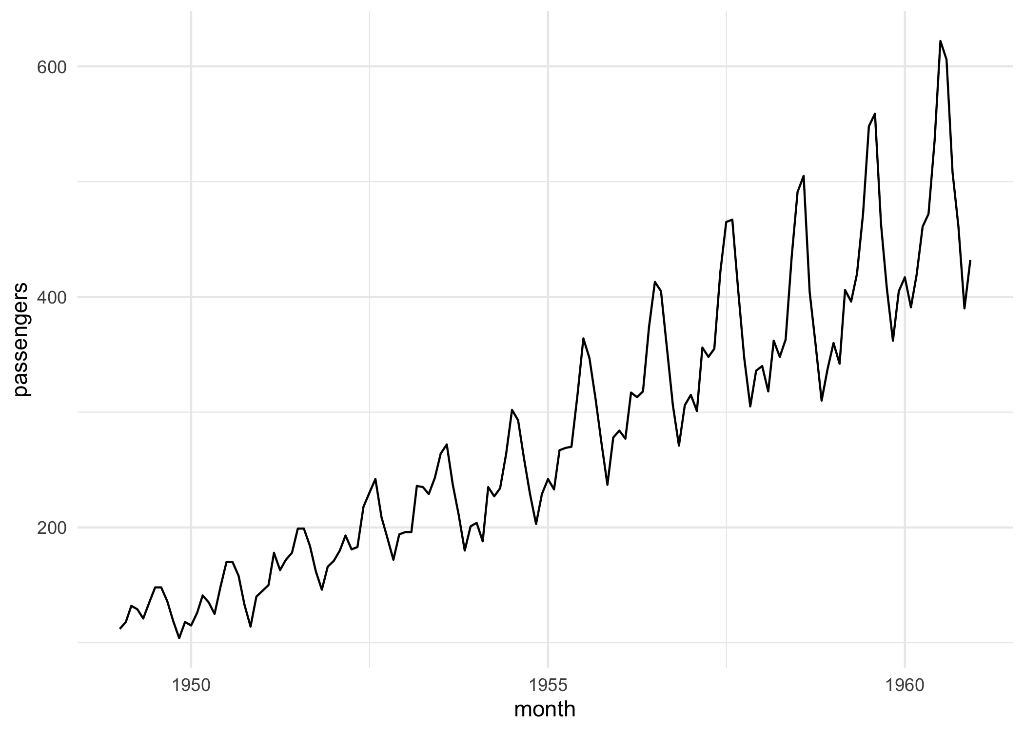
# train a forecast learner
learner = lrn("fcst.auto_arima")$train(task)
prediction = learner$predict(task, 140:144)
prediction
#>
#> ── <PredictionFcst> for 5 observations: ────────────────────────────────────────
#>       month row_ids truth response
#>  1960-08-01     140   606 623.9219
#>  1960-09-01     141   508 513.8585
#>  1960-10-01     142   461 450.7762
#>  1960-11-01     143   390 410.8961
#>  1960-12-01     144   432 439.9462
prediction$score(msr("regr.rmse"))
#> regr.rmse
#>  13.85518
To forecast beyond the observed data, generate_newdata()
builds the future rows (with missing targets) and
predict_newdata() fills them in:
# generate new data to forecast unseen data
newdata = generate_newdata(task, 12L)
head(newdata)
#>         month passengers
#> 1: 1961-01-01         NA
#> 2: 1961-02-01         NA
#> 3: 1961-03-01         NA
#> 4: 1961-04-01         NA
#> 5: 1961-05-01         NA
#> 6: 1961-06-01         NA
prediction = learner$predict_newdata(newdata, task)
prediction
#>
#> ── <PredictionFcst> for 12 observations: ───────────────────────────────────────
#>       month row_ids truth response
#>  1961-01-01       1    NA 445.6351
#>  1961-02-01       2    NA 420.3953
#>  1961-03-01       3    NA 449.1988
#>         ---     ---   ---      ---
#>  1961-10-01      10    NA 494.1275
#>  1961-11-01      11    NA 423.3336
#>  1961-12-01      12    NA 465.5085
The forecast() helper combines these two steps,
generating the future rows and predicting them in a single call:
prediction = forecast(learner, task, 12L)
prediction
#>
#> ── <PredictionFcst> for 12 observations: ───────────────────────────────────────
#>       month row_ids truth response
#>  1961-01-01       1    NA 445.6351
#>  1961-02-01       2    NA 420.3953
#>  1961-03-01       3    NA 449.1988
#>         ---     ---   ---      ---
#>  1961-10-01      10    NA 494.1275
#>  1961-11-01      11    NA 423.3336
#>  1961-12-01      12    NA 465.5085
The resulting PredictionFcst
can be plotted with autoplot(), overlaying the forecast on
the historical series:
autoplot(prediction, task)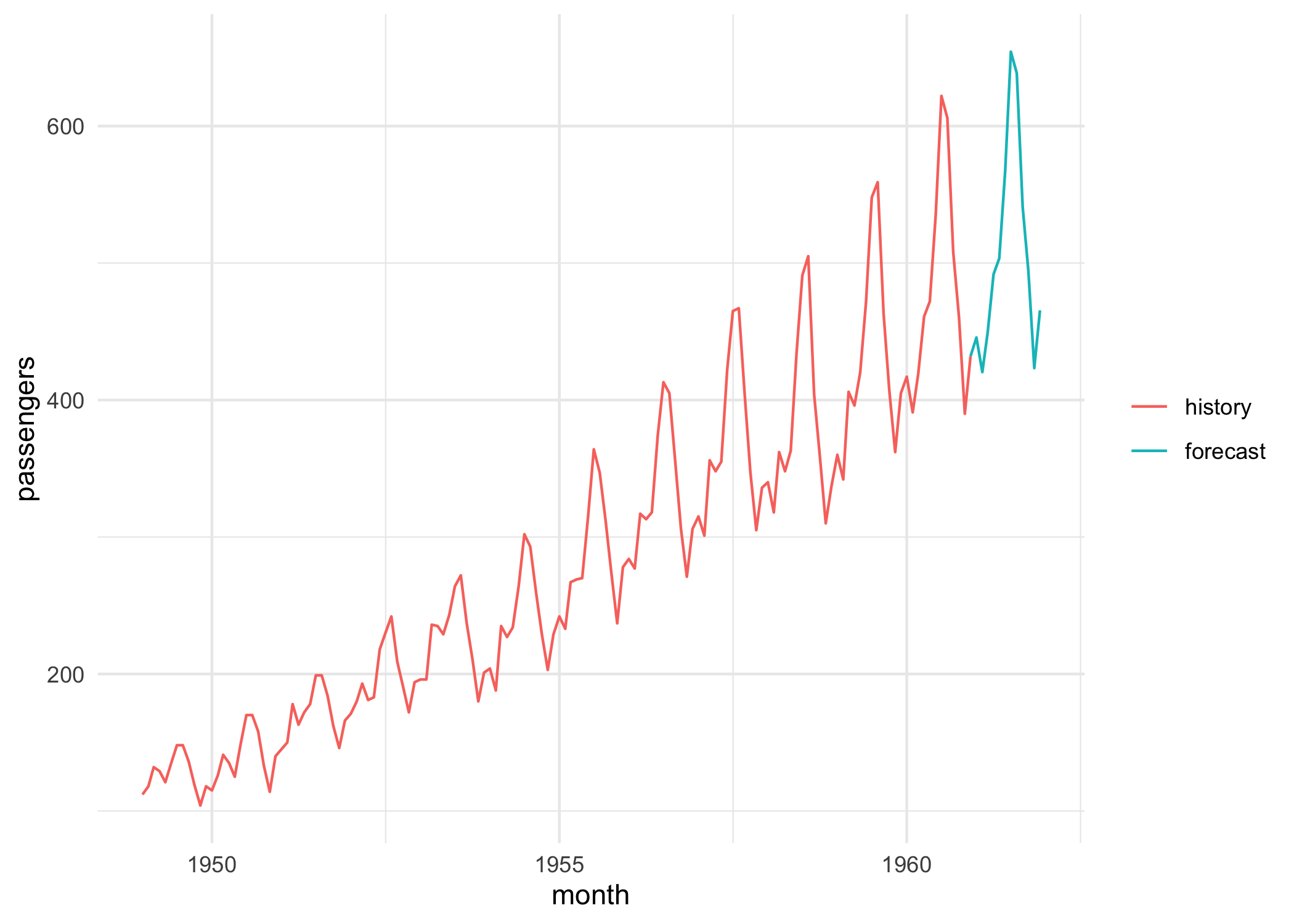
Target transformations can be applied by wrapping the learner in
ppl("targettrafo"):
# add a target log transformation
learner = as_learner(ppl(
  "targettrafo",
  graph = lrn("fcst.auto_arima"),
  targetmutate.trafo = function(x) log(x),
  targetmutate.inverter = function(x) list(response = exp(x$response))
))
prediction = learner$train(task)$predict(task, 140:144)
prediction$score(msr("regr.rmse"))
#> regr.rmse
#>  12.29896
Which predict types a learner supports
(e.g. "quantiles", "se") is listed in its
predict_types:
lrn("fcst.auto_arima")$predict_types
#> [1] "response"  "quantiles"
Classical forecasters can then return a predictive distribution as quantiles, scored with probabilistic measures such as the Pinball loss:
# works with quantile response
learner = lrn(
  "fcst.auto_arima",
  predict_type = "quantiles",
  quantiles = c(0.1, 0.15, 0.5, 0.85, 0.9),
  quantile_response = 0.5
)$train(task, 1:132)
prediction = learner$predict(task, 133:144)
prediction
#>
#> ── <PredictionFcst> for 12 observations: ───────────────────────────────────────
#>       month row_ids truth     q0.1    q0.15     q0.5    q0.85     q0.9 response
#>  1960-01-01     133   417 410.6811 413.2496 424.1099 434.9702 437.5387 424.1099
#>  1960-02-01     134   391 390.2142 393.4355 407.0557 420.6759 423.8972 407.0557
#>  1960-03-01     135   419 450.7334 454.5764 470.8257 487.0751 490.9181 470.8257
#>         ---     ---   ---      ---      ---      ---      ---      ---      ---
#>  1960-10-01     142   461 436.9438 443.6242 471.8707 500.1173 506.7976 471.8707
#>  1960-11-01     143   390 390.3115 397.3040 426.8707 456.4374 463.4300 426.8707
#>  1960-12-01     144   432 431.7490 439.0404 469.8707 500.7011 507.9925 469.8707
prediction$score(msr("fcst.pinball"))
#> fcst.pinball
#>     11.38111
Forecasting resamplings respect the temporal order of the observations:
# resampling, scored with a forecasting measure (MASE)
learner = lrn("fcst.auto_arima")
resampling = rsmp("fcst.holdout", ratio = 0.7)
rr = resample(task, learner, resampling)
rr$aggregate(msrs(c("regr.rmse", "fcst.mase")))
#> regr.rmse fcst.mase
#> 27.121096 1.212049Any regression learner can be turned into a forecaster with
recursive_forecaster(), which adds lag features and
forecasts recursively:
library(mlr3learners)

task = tsk("airpassengers")
learner = lrn("regr.ranger")
flrn = recursive_forecaster(learner, lags = 1:12)$train(task)
newdata = generate_newdata(task, 12L)
prediction = flrn$predict_newdata(newdata, task)
prediction
#>
#> ── <PredictionFcst> for 12 observations: ───────────────────────────────────────
#>       month row_ids truth response
#>  1961-01-01       1    NA 444.8088
#>  1961-02-01       2    NA 445.5287
#>  1961-03-01       3    NA 466.5617
#>         ---     ---   ---      ---
#>  1961-10-01      10    NA 488.7945
#>  1961-11-01      11    NA 458.7724
#>  1961-12-01      12    NA 461.9348
prediction = flrn$predict(task, 140:144)
prediction
#>
#> ── <PredictionFcst> for 5 observations: ────────────────────────────────────────
#>       month row_ids truth response
#>  1960-08-01     140   606 565.3158
#>  1960-09-01     141   508 504.3124
#>  1960-10-01     142   461 460.2565
#>  1960-11-01     143   390 419.6708
#>  1960-12-01     144   432 441.9507
prediction$score(msr("regr.rmse"))
#> regr.rmse
#>  23.01621

flrn = recursive_forecaster(learner, lags = 1:12)
resampling = rsmp("fcst.holdout", ratio = 0.9)
rr = resample(task, flrn, resampling)
rr$aggregate(msr("regr.rmse"))
#> regr.rmse
#>   52.2975

resampling = rsmp("fcst.cv")
rr = resample(task, flrn, resampling)
rr$aggregate(msr("regr.rmse"))
#> regr.rmse
#> 38.83575recursive_forecaster() builds a recursive forecaster
(one model, applied iteratively). Use direct_forecaster()
with horizons to train one model per horizon instead —
predictions then come straight from each horizon’s model, with no error
accumulation:
task = tsk("airpassengers")
flrn = direct_forecaster(
  lrn("regr.ranger"),
  lags = 1:12,
  horizons = 12
)$train(task, 1:132)
flrn$predict(task, 133:144)$score(msr("regr.rmse"))
#> regr.rmse
#> 55.29949Lag features can be combined with other transformations using mlr3pipelines:
library(mlr3pipelines)

task = tsk("airpassengers")
task$set_col_roles("month", add = "feature")
graph = po("fcst.lags", lags = 1:12) %>>%
  po(
    "datefeatures",
    param_vals = list(
      week_of_year = FALSE,
      day_of_year = FALSE,
      day_of_month = FALSE,
      day_of_week = FALSE
    )
  ) %>>%
  lrn("regr.ranger")
flrn = recursive_forecaster(graph)$train(task)
prediction = flrn$predict(task, 142:144)
prediction$score(msr("regr.rmse"))
#> regr.rmse
#>  15.64558
Use selector_fcst_lags() to apply transformations only
to the lag features, e.g. log-transforming lags while leaving date
features untouched:
task = tsk("airpassengers")
task$set_col_roles("month", add = "feature")
graph = po("fcst.lags", lags = 1:12) %>>%
  po("colapply", applicator = log, affect_columns = selector_fcst_lags()) %>>%
  po(
    "datefeatures",
    param_vals = list(
      week_of_year = FALSE,
      day_of_year = FALSE,
      day_of_month = FALSE,
      day_of_week = FALSE
    )
  ) %>>%
  lrn("regr.ranger")
flrn = recursive_forecaster(graph)$train(task)
prediction = flrn$predict(task, 142:144)
prediction$score(msr("regr.rmse"))
#> regr.rmse
#>  20.86682
Target transformations can be applied by wrapping the forecast
learner in ppl("targettrafo"). The lags are created from
the transformed target and predictions are automatically inverted back
to the original scale:
task = tsk("airpassengers")
graph = po("fcst.lags", lags = 1:12) %>>% lrn("regr.ranger")
pipeline = ppl(
  "targettrafo",
  graph = recursive_forecaster(graph),
  targetmutate.trafo = function(x) log(x),
  targetmutate.inverter = function(x) list(response = exp(x$response))
)
learner = as_learner(pipeline)$train(task)
prediction = learner$predict(task, 142:144)
prediction$score(msr("regr.rmse"))
#> regr.rmse
#>  14.36929
Ready-made po("fcst.targetboxcox") and
po("fcst.targetdiff") pipeops are also available for
Box-Cox transformation and differencing.
Forecasting tasks can include exogenous covariates. Here electricity demand is forecast from its own lags, calendar features, and external regressors (temperature, holiday) supplied for the forecast horizon:
library(mlr3learners)
library(mlr3pipelines)

task = tsk("electricity")
task$set_col_roles("date", add = "feature")
graph = po("fcst.lags", lags = 1:3) %>>%
  po("datefeatures", param_vals = list(year = FALSE)) %>>%
  lrn("regr.ranger")
flrn = recursive_forecaster(graph)$train(task)

max_date = task$data()[.N, date]
newdata = data.table(
  date = max_date + 1:14,
  demand = rep(NA_real_, 14L),
  temperature = 26,
  holiday = c(TRUE, rep(FALSE, 13L))
)
prediction = flrn$predict_newdata(newdata, task)
prediction
#>
#> ── <PredictionFcst> for 14 observations: ───────────────────────────────────────
#>        date row_ids truth response
#>  2015-01-01       1    NA 187879.1
#>  2015-01-02       2    NA 196579.6
#>  2015-01-03       3    NA 192664.9
#>         ---     ---   ---      ---
#>  2015-01-12      12    NA 222994.8
#>  2015-01-13      13    NA 227703.9
#> 2015-01-14 14 NA 228434.0ML forecasters declare task_type = "fcst", so they can
be benchmarked side-by-side with classical learners on the same task in
a single benchmark() call:
task = tsk("airpassengers")
resampling = rsmp("fcst.holdout", ratio = 0.9)$instantiate(task)
n_test = length(resampling$test_set(1L))

learners = list(
  lrn("fcst.arima", id = "arima"),
  recursive_forecaster(lrn("regr.ranger"), lags = 1:12, id = "ranger_recursive"),
  direct_forecaster(
    lrn("regr.ranger"),
    lags = 1:12,
    horizons = n_test,
    id = "ranger_direct"
  )
)
design = benchmark_grid(task, learners, resampling)
bmr = benchmark(design)
bmr$aggregate(msr("regr.rmse"))[, .(learner_id, regr.rmse)]
#>          learner_id regr.rmse
#> 1:            arima 216.31005
#> 2: ranger_recursive  49.73233
#> 3: ranger_direct 52.65376Several forecasters can be ensembled by branching with
gunion() and averaging their forecasts with
po("fcst.avg"), which keeps the forecast prediction type
(so the time index, keys, and autoplot() survive the
averaging). This mirrors the idea behind the forecastHybrid package, but
with any mix of classical or ML learners.
task = tsk("airpassengers")

graph = gunion(list(
  po("learner", lrn("fcst.auto_arima"), id = "arima"),
  po("learner", lrn("fcst.ets"), id = "ets"),
  po("learner", lrn("fcst.theta"), id = "theta")
)) %>>%
  po("fcst.avg")
flrn = as_learner(graph)$train(task)
forecast(flrn, task, 12L)
#>
#> ── <PredictionFcst> for 12 observations: ───────────────────────────────────────
#>       month row_ids truth response
#>  1961-01-01       1    NA 442.5050
#>  1961-02-01       2    NA 427.6327
#>  1961-03-01       3    NA 478.5120
#>         ---     ---   ---      ---
#>  1961-10-01      10    NA 471.2626
#>  1961-11-01      11    NA 408.0117
#>  1961-12-01      12    NA 455.0409
flrn$predict(task, 140:144)$score(msr("regr.rmse"))
#> regr.rmse
#>  12.23143

# weight the members instead of averaging equally
graph$param_set$set_values(fcst.avg.weights = c(0.5, 0.3, 0.2))
flrn = as_learner(graph)$train(task)
flrn$predict(task, 140:144)$score(msr("regr.rmse"))
#> regr.rmse
#> 12.28049Forecast learners are regular mlr3 learners, so they plug into the
standard mlr3tuning
machinery. Mark hyperparameters with to_tune() and wrap the
learner in an auto_tuner(), using a forecasting resampling
such as fcst.holdout or fcst.cv to respect the
temporal order:
library(mlr3tuning)

task = tsk("airpassengers")

# tune an ML forecaster
flrn = recursive_forecaster(lrn("regr.ranger"), lags = 1:12)
flrn$param_set$set_values(
  regr.ranger.mtry.ratio = to_tune(0.1, 1),
  regr.ranger.num.trees = to_tune(100, 500)
)
at = auto_tuner(
  tuner = tnr("random_search"),
  learner = flrn,
  resampling = rsmp("fcst.cv"),
  measure = msr("regr.rmse"),
  term_evals = 4
)
at$train(task)
at$tuning_result[, .(regr.ranger.mtry.ratio, regr.ranger.num.trees, regr.rmse)]
#>    regr.ranger.mtry.ratio regr.ranger.num.trees regr.rmse
#> 1:              0.7081945                   309  25.65191

# the AutoTuner is itself a learner: predict with the best configuration
at$predict(task, 142:144)$score(msr("regr.rmse"))
#> regr.rmse
#>  10.16563
Classical forecasters tune the same way:
flrn = lrn("fcst.auto_arima")
flrn$param_set$set_values(stationary = to_tune(p_lgl()), seasonal = to_tune(p_lgl()))
at = auto_tuner(
  tuner = tnr("grid_search"),
  learner = flrn,
  resampling = rsmp("fcst.holdout", ratio = 0.8),
  measure = msr("regr.rmse")
)
at$train(task)
at$tuning_result[, .(stationary, seasonal, regr.rmse)]
#>    stationary seasonal regr.rmse
#> 1: FALSE TRUE 35.08279In machine learning forecasting the difference between forecasting a
single time series and longitudinal data is often referred to as local
and global forecasting. A global model is trained jointly across many
series, identified by a key:
library(mlr3learners)
library(mlr3pipelines)
library(tsibble)

dt = setDT(tsibbledata::aus_livestock)
setnames(dt, tolower)
dt[, month := as.Date(month)]
dt = dt[, .(count = sum(count)), by = .(state, month)]
setorder(dt, state, month)
task = as_task_fcst(dt, id = "aus_livestock", target = "count", order = "month", key = "state", freq = "month")
task$set_col_roles("month", add = "feature")

graph = po("fcst.lags", lags = 1:12) %>>%
  po(
    "datefeatures",
    param_vals = list(
      week_of_year = FALSE,
      day_of_week = FALSE,
      day_of_month = FALSE,
      day_of_year = FALSE
    )
  ) %>>%
  lrn("regr.ranger")

flrn = recursive_forecaster(graph)$train(task)
prediction = flrn$predict(task, 4460:4464)
prediction$score(msr("regr.rmse"))
#> regr.rmse
#>  18531.79

resampling = rsmp("fcst.holdout", ratio = 0.9)
rr = resample(task, flrn, resampling)
rr$aggregate(msr("regr.rmse"))
#> regr.rmse
#> 103746.2A single global model can be compared against fitting one local model per series:
retail = setDT(tsibbledata::aus_retail)
setnames(retail, tolower)
retail[, month := as.Date(month)]
vic = retail[state == "Victoria"]
vic[, let(state = NULL, `series id` = NULL)]
vic[, industry := as.factor(industry)]
vic_train = vic[month < as.Date("2015-01-01")]
vic_test = vic[month >= as.Date("2015-01-01")]

# global forecasting
task_train = as_task_fcst(
  vic_train,
  id = "aus_retail_vic",
  target = "turnover",
  order = "month",
  key = "industry",
  freq = "month"
)
task_test = as_task_fcst(
  vic_test,
  id = "aus_retail_vic",
  target = "turnover",
  order = "month",
  key = "industry",
  freq = "month"
)

learner = lrn("regr.ranger", verbose = FALSE)
flrn = recursive_forecaster(learner, lags = 1:12)$train(task_train)
prediction_global = flrn$predict(task_test)
prediction_global
#>
#> ── <PredictionFcst> for 960 observations: ──────────────────────────────────────
#>                                  industry      month row_ids truth response
#>  Cafes, restaurants and catering services 2015-01-01       1 476.2 467.7033
#>  Cafes, restaurants and catering services 2015-02-01       2 422.0 456.7255
#>  Cafes, restaurants and catering services 2015-03-01       3 471.2 488.5871
#>                                       ---        ---     ---   ---      ---
#>                    Takeaway food services 2018-10-01     958 359.2 397.7645
#>                    Takeaway food services 2018-11-01     959 354.9 403.2076
#>                    Takeaway food services 2018-12-01     960 393.2 411.0413
prediction_global$score(msr("regr.rmse"))
#> regr.rmse
#>  83.95134

# local forecasting
prediction_local = map(split(vic, by = "industry", drop = TRUE), function(dt) {
  task_train = as_task_fcst(
    dt[month < as.Date("2015-01-01")],
    id = "aus_retail_vic_local",
    target = "turnover",
    order = "month",
    freq = "month"
  )
  task_test = as_task_fcst(
    dt[month >= as.Date("2015-01-01")],
    id = "aus_retail_vic_local",
    target = "turnover",
    order = "month",
    freq = "month"
  )
  flrn = recursive_forecaster(learner, lags = 1:12)$train(task_train)
  prediction = flrn$predict(task_test)
  prediction
})
do.call(c, prediction_local)$score(msr("regr.rmse"))
#> regr.rmse
#>  95.72716