potentiomap

potentiomap builds potentiometric surface products from groundwater monitoring data. It prepares groundwater elevation observations from direct water-level measurements or depth-to-water measurements, interpolates a continuous potentiometric surface, generates contour products, and derives hydraulic gradient flow arrows suitable for GIS review and technical reporting.

The default interpolation method is a thin-plate spline (TPS), which provides a smooth surface appropriate for many monitoring-well networks. Additional built-in methods include inverse distance weighting (IDW), ordinary kriging (OK), and universal kriging (UK). Advanced users can also supply their own interpolation function.

Installation

Install the released version:

install.packages("potentiomap")

Install the development version:

install.packages("remotes")
remotes::install_github("el-cordero/potentiomap")

Load the package:

library(potentiomap)
library(terra)

Core Workflow

potentiomap organizes a groundwater surface workflow into four stages:

1. Prepare monitoring points with a standardized groundwater elevation field.
2. Interpolate a potentiometric surface on a raster grid.
3. Export surface, contour, and quicklook products.
4. Generate hydraulic-gradient arrows and arrow-tip or arrow-base point layers.

The package accepts coordinate tables, sf objects, and terra::SpatVector point layers. Tabular inputs require coordinate columns and a coordinate reference system.

Example Data

The package includes synthetic example data for reproducible examples:

• synthetic_wells: monitoring-well coordinates, land-surface elevations, depth-to-water measurements, and groundwater elevations.
• synthetic_dem: a packed terra raster representing land-surface elevation.
• synthetic_surface_points: separate land-surface elevation measurements.
• ps_sample_aoi(): an example area-of-interest polygon.

data("synthetic_wells")
data("synthetic_dem")
data("synthetic_surface_points")

synthetic_dem <- terra::rast(synthetic_dem)

Preparing Groundwater Elevation Points

Direct Groundwater Elevation Measurements

Use ps_make_points() when groundwater elevation is already present in the input table.

gw_points <- ps_make_points(
  synthetic_wells,
  x = "x",
  y = "y",
  value = "gw_elevation",
  name_col = "well_id",
  crs = "EPSG:26916"
)

The returned point layer contains standardized Z and Name fields. Z is the groundwater elevation used by the interpolation functions.

Depth to Water with a DEM

Use ps_potentiometric_points() when field data contain depth to water and land-surface elevation should be sampled from a DEM.

gw_points <- ps_potentiometric_points(
  synthetic_wells,
  x = "x",
  y = "y",
  depth_col = "depth_to_water",
  surface = synthetic_dem,
  name_col = "well_id",
  crs = "EPSG:26916"
)

Depth to Water with a Surface-Elevation Column

If the well table already contains land-surface elevation, provide that column through surface_col.

gw_points <- ps_potentiometric_points(
  synthetic_wells,
  x = "x",
  y = "y",
  depth_col = "depth_to_water",
  surface_col = "surface_elevation",
  name_col = "well_id",
  crs = "EPSG:26916"
)

Depth to Water with Separate Surface Points

Separate land-surface elevation points can also be used. Matching names are used when available; otherwise the surface elevation points are interpolated to the groundwater measurement locations.

gw_points <- ps_potentiometric_points(
  synthetic_wells,
  x = "x",
  y = "y",
  depth_col = "depth_to_water",
  surface = synthetic_surface_points,
  surface_col = "surface_elevation",
  name_col = "well_id",
  surface_name_col = "point_id",
  crs = "EPSG:26916"
)

Interpolation

The default call uses thin-plate spline interpolation.

tps_surface <- ps_interpolate(
  gw_points,
  grid_res = 50,
  mask = ps_sample_aoi()
)

names(tps_surface)

Run multiple built-in methods by passing methods.

surfaces <- ps_interpolate(
  gw_points,
  methods = c("TPS", "IDW", "OK", "UK"),
  grid_res = 50,
  mask = ps_sample_aoi(),
  padding = 150
)

Custom Interpolation Methods

Custom methods receive the prepared point layer, the template raster, and the prediction grid. They must return either a terra::SpatRaster matching the template or a numeric vector with one value per template cell.

mean_surface <- function(points, template, grid) {
  rep(mean(terra::values(points)$Z), terra::ncell(template))
}

custom_surface <- ps_interpolate(
  gw_points,
  methods = "mean_surface",
  custom_methods = list(mean_surface = mean_surface),
  grid_res = 50,
  mask = ps_sample_aoi()
)

Exporting Surface Products

ps_export_surfaces() writes GeoTIFF surfaces, contour shapefiles, and quicklook PNG figures.

out_dir <- file.path(tempdir(), "potentiomap-products")

outputs <- ps_export_surfaces(
  surfaces,
  points = gw_points,
  out_dir = out_dir,
  out_stub = "synthetic",
  contour_interval = 1
)

outputs

The output table lists the raster, contour, and quicklook file paths for each interpolation method.

Surface Smoothing

Interpolated surfaces sometimes contain local roughness that is not useful for contour development or gradient visualization. ps_smooth_surface() applies a focal moving-window smoother to the raster while preserving the original raster geometry and, by default, the original NA footprint.

smoothed_tps <- ps_smooth_surface(
  surfaces$TPS,
  window_size = 5,
  method = "mean",
  iterations = 2
)

smoothed_contours <- ps_contours(smoothed_tps, interval = 1)

The smoothing function can be used before contour extraction or before hydraulic-gradient arrow development when a smoother display product is needed.

Hydraulic Gradient and Flow Arrows

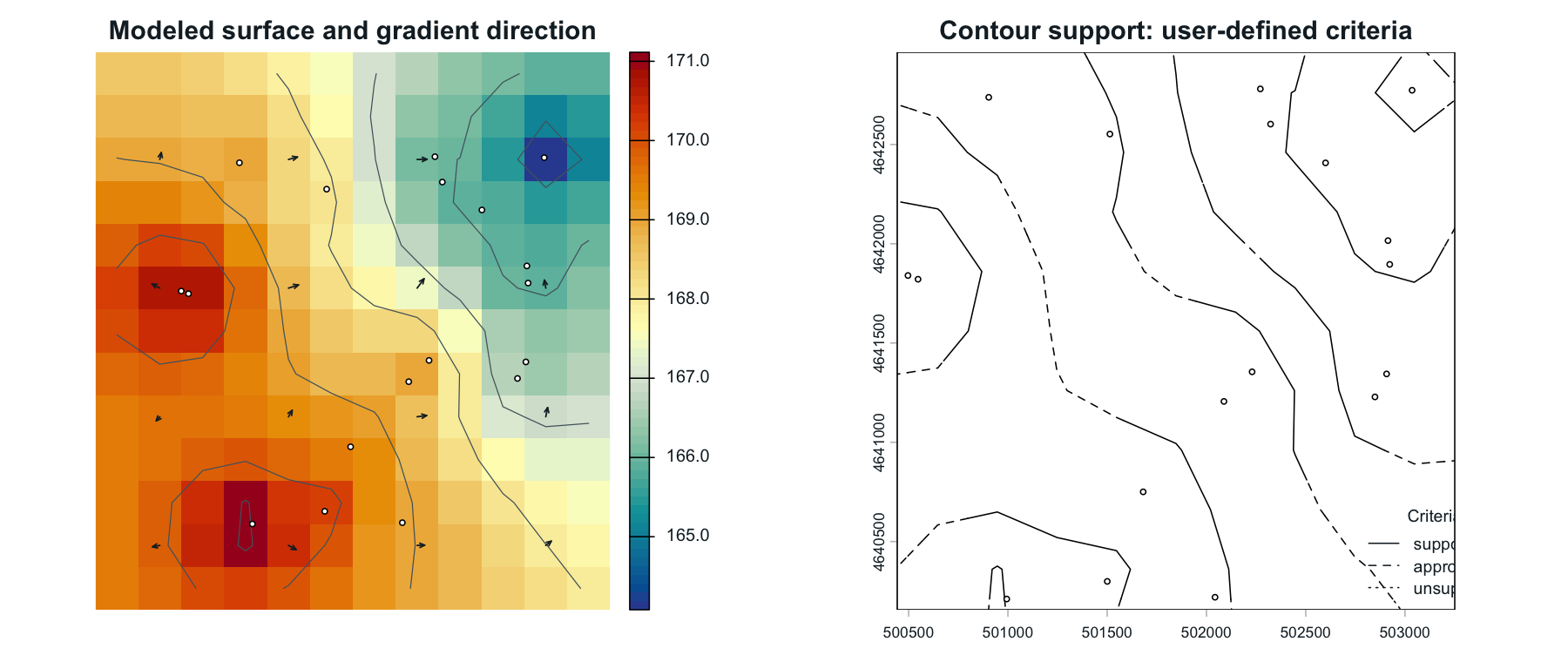
ps_flow_arrows() calculates slope and aspect from a potentiometric surface, converts slope to hydraulic gradient, samples the gradient to a readable arrow spacing, and builds downgradient line features.

flow <- ps_flow_arrows(
  surfaces$TPS,
  res_factor = 8,
  scale = 80,
  out_dir = out_dir,
  out_stub = "synthetic_TPS"
)

tips <- ps_arrow_vertices(
  flow$arrows,
  which = "last",
  out_file = file.path(out_dir, "synthetic_TPS_arrow_tips.shp")
)

bases <- ps_arrow_vertices(
  flow$arrows,
  which = "first",
  out_file = file.path(out_dir, "synthetic_TPS_arrow_bases.shp")
)

The flow output includes a hydraulic-gradient raster, sampled gradient points, arrow lines, arrow tips, and arrow bases.

Visual Examples

The following panels are generated from the bundled synthetic dataset. Each figure uses one row and four columns to show how an output changes as one modeling or display choice varies.

Interpolation Method

TPS is the default method. IDW, OK, and UK are available when comparison among surface assumptions is useful.

Grid Resolution

Smaller grid cells preserve more local detail but create larger output rasters. Coarser grids are faster and may be appropriate for broad screening maps.

Contour Interval

Contour interval controls how much vertical detail is shown. Fine intervals can highlight subtle gradients; wider intervals can make regional patterns easier to read.

TPS Smoothing

TPS smoothing can be selected automatically by generalized cross-validation or specified directly through tps_lambda.

Raster Smoothing

ps_smooth_surface() can be applied after interpolation when a smoother surface is desirable for contours or arrows.

Arrow Density

res_factor controls the spacing of sampled hydraulic-gradient arrows. Higher values create fewer arrows; lower values create denser arrow fields.

Arrow Scale

scale controls arrow length. Larger values emphasize small gradients; smaller values reduce visual clutter.

Choosing a Method

TPS is a practical default for producing smooth potentiometric surfaces from typical monitoring-well datasets. IDW is deterministic and easy to interpret. Kriging methods can be valuable when the observation network supports a meaningful variogram model, but sparse monitoring networks may produce variogram-fit warnings. Those warnings should be reviewed as part of model selection rather than suppressed automatically.

References

Hijmans, R. J. 2025. terra: Spatial data analysis. R package version 1.9-1. https://doi.org/10.32614/CRAN.package.terra

Nychka, D., R. Furrer, J. Paige, and S. Sain. 2021. fields: Tools for spatial data. R package version 17.1. https://doi.org/10.5065/D6W957CT

Pebesma, E. 2004. Multivariable geostatistics in S: The gstat package. Computers & Geosciences 30:683-691. https://doi.org/10.1016/j.cageo.2004.03.012