![]()
![]()
The goal of ssrn is to implement the algorithm provided in “Scan for estimating the transmission route of COVID-19 on railway network using passenger volume”. It is a generalization of the scan statistic approach for railway network to identify the hot railway route for transmitting infectious diseases.
You can install the development version of ssrn from GitHub with:
if (!requireNamespace("remotes"))
  install.packages("remotes")

remotes::install_github("uribo/ssrn")Below are some of the features of the package, using the built-in dataset (a section of JR’s Tokaido Line).
library(ssrn)
library(scanstatistics)
library(dplyr)
data("jreast_jt", package = "ssrn")
jreast_jt includes the code and names of stations
between Tokyo and Yugawara.
glimpse(jreast_jt)
#> Rows: 20
#> Columns: 2
#> $ st_code <chr> "00101", "00102", "00103", "00104", "00105", "00106", "00107"…
#> $ st_name <chr> "Tokyo", "Shimbashi", "Shinagawa", "Kawasaki", "Yokohama", "T…
glimpse(jreast_jt_od)
#> Rows: 197
#> Columns: 4
#> $ rw_code           <chr> "001", "001", "001", "001", "001", "001", "001", "0…
#> $ departure_st_code <chr> "00101", "00101", "00101", "00101", "00101", "00101…
#> $ arrive_st_code    <chr> "00102", "00103", "00104", "00105", "00106", "00107…
#> $ volume <dbl> 950, 1690, 3447, 2387, 542, 459, 271, 377, 597, 859…Prepare a matrix object to detect hotspots from spatial relationships on the railway. This package provides auxiliary functions that create these matrices based on the data indicating the relationship between stations (the order of stops) and the passenger volumes.
make_adjacency_matrix().make_passenger_matrix()
based on the passenger volumes.network_window() set the zone from the railway
network.adj <-
make_adjacency_matrix(jreast_jt,
st_code, next_st_code)
dist <-
jreast_jt_od %>%
make_passenger_matrix(jreast_jt,
departure_st_code,
arrive_st_code,
st_code,
volume)zones <-
network_window(adj,
dist,
type = "connected_B",
cluster_max = 20)zones
#> [[1]]
#> [1] 1
#>
#> [[2]]
#> [1] 1 2
#>
#> [[3]]
#> [1] 1 2 3
#>
#> [[4]]
#> [1] 1 2 3 4
#> ...
#> [[134]]
#> [1] 20Apply the method of spatial scan statistics based on the zone. Here’s an example of applying dummy data in the scanstatistics.
counts <-
  c(2, 2, 1, 5, 7, 1,
    1, 1, 1, 1, 2, 2,
    5, 4, 7, 5, 1, 2,
    1, 1) %>%
  purrr::set_names(
    jreast_jt$st_name)
counts
#>      Tokyo  Shimbashi  Shinagawa   Kawasaki   Yokohama    Totsuka      Ofuna
#>          2          2          1          5          7          1          1
#>   Fujisawa    Tsujido  Chigasaki  Hiratsuka       Oiso   Ninomiya       Kozu
#>          1          1          1          2          2          5          4
#> Kamonomiya    Odawara   Hayakawa   Nebukawa   Manazuru   Yugawara
#>          7          5          1          2          1          1

poisson_result <-
  scan_eb_poisson(counts = counts,
                  zones = zones,
                  baselines = rep(1, 20),
                  n_mcsim = 10000,
                  max_only = FALSE)
top <- top_clusters(poisson_result,
zones,
k = 2,
overlapping = FALSE)
detect_zones <-
top$zone %>%
purrr::map(get_zone, zones = zones) %>%
purrr::map(function(x) jreast_jt$st_name[x])
df_zones <-
seq_len(length(detect_zones)) %>%
purrr::map_df(
~ tibble::tibble(
cluster = .x,
st_name = detect_zones[.x]
)
) %>%
tidyr::unnest(cols = st_name)
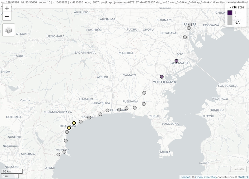
df_zones
#> # A tibble: 4 x 2
#> cluster st_name
#> <int> <chr>
#> 1 1 Kawasaki
#> 2 1 Yokohama
#> 3 2 Kamonomiya
#> 4 2 Odawara