ade4 in
Ecological Data Analysis : Exploratory and Euclidean methods in Environmental sciences

Article Rnews 2007

The ade4 package - II: Two-table and {K}-table methods

The ade4 package - II: Two-table and K-table methods

by Stéphane Dray, Anne B. Dufour and Daniel Chessel

S. Dray, A.B. Dufour, and D. Chessel. 2007. The ade4 package - II: Two-table and K-table methods. R News 7(2):47-52.

Introduction
Ecological illustration
Matching two tables
The K-table class
Conclusion

1 Introduction

The ade4 package proposes a great variety of explanatory methods to analyse multivariate datasets. As suggested by the acronym ade4 (Data Analysis functions to analyse Ecological and Environmental data in the framework of Euclidean Exploratory methods), the package is devoted to ecologists but it could be useful in many other fields [e.g.,Goecke, 2005]. Methods available in the package are particular cases of the duality diagram [Escoufier, 1987,Holmes, 2006,Dray and Dufour, 2007] and the implementation of the functions follows the description of this unifying mathematical tool (class dudi). The main functions of the package for one-table analysis methods have been presented in Chessel et al. [2004]. This new paper presents a short summary of two-table and K-table methods available in the package.

2 Ecological illustration

In order to illustrate the methods, we used the dataset jv73 [Verneaux, 1973] which is available in the package. This dataset concerns 12 rivers. For each river, a number of sites have been sampled. The number of sites per river is not constant. jv73$poi is a data.frame and contains presence / absence data for 19 fish species (columns) in 92 sites (rows). jv73$fac.riv is a factor indicating the river corresponding to each site. jv73$morpho contains the measurements of six environmental variables (altitude (m), distance between the site and the source (km), slope (per thousand), wetted cross section (m²), average flow (m³/s) and average speed (m/s)) for the same sites . Several ecological questions are related to these data:

Are they groups of fish species living together (i.e. species communities)?
Is there a relation between the composition of fish communities and the environmental variations?
Does the composition of fish communities vary (or not) among rivers?
Do the species-environment relationships vary (or not) among rivers?

Multivariate analyses help to answer these different questions: one-table methods for the first question, two-table methods for the second one and K-table methods for the last two ones.

3 Matching two tables

The main purpose of ecological data analysis is the matching of two data tables: a sites-by-environmental variables table and a sites-by-species table, to study the relationships between the composition of species communities and their environment. The ade4 package contains the main variants of these methods (procrustean rotation, co-inertia analysis and principal component analyses with respect to instrumental variables).

The first approach is procrustean rotation [Gower, 1971], introduced in ecology by [Digby and Kempton, 1987, p. 116].

 data(jv73)
 pca1 <- dudi.pca(jv73$morpho, scannf = FALSE)
 pca2 <- dudi.pca(jv73$poi, scale = FALSE, 
     scannf = FALSE)
 plot(procuste(pca1$tab, pca2$tab, 
     nf = 2))

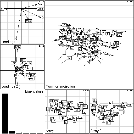Figure 1: Plot of a Procrustes analysis: loadings for environmental variables and species, eigenvalues screeplot, scores of sites for the two data sets, and projection of the two sets of sites after rotation (arrows link environment site score to the species site score) [Dray et al., 2003a].

Two randomization procedures are available to test the association between two tables: PROTEST [Jackson, 1995] and RV [Heo and Gabriel, 1998].

 plot(procuste.randtest(pca1$tab, 
     pca2$tab), main = "PROTEST")

 plot(RV.rtest(pca1$tab, pca2$tab), 
     main = "RV")

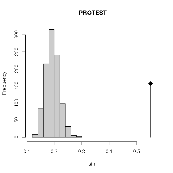
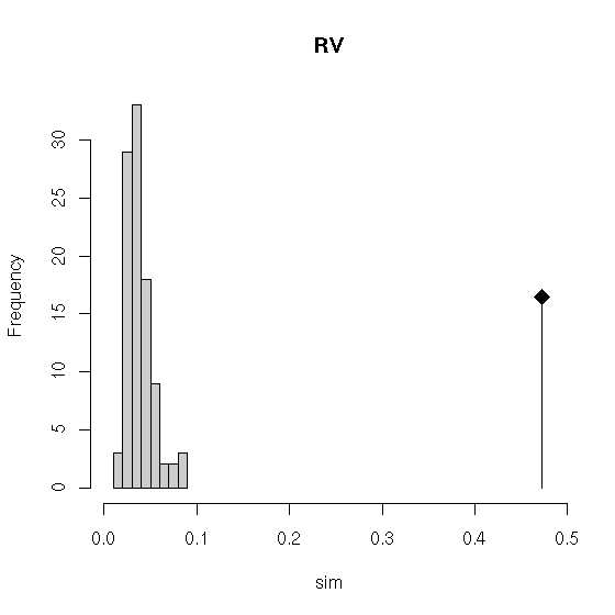Figure 2: Plots of PROTEST and RV tests: histograms of simulated values and observed value (vertical line).

Co-inertia analysis [Dolédec and Chessel, 1994,Dray et al., 2003b] is a general approach that can be applied to any pair of duality diagrams having the same row weights. This method is symmetric and seeks for a common structure between two datasets. It extends psychometricians inter-battery analysis [Tucker, 1958], canonical analysis on qualitative variables [Cazes, 1980], and ecological profiles analysis [Montaña and Greig-Smith, 1990,Mercier et al., 1992]. Co-inertia analysis of the pair of triplets (X₁,Q₁,D) and (X₂,Q₂,D) leads to the triplet (X₂^tDX₁,Q₁,Q₂). Note that the two triplets must have the same row weights.

 coa1 <- dudi.coa(jv73$poi, scannf = FALSE)
 pca3 <- dudi.pca(jv73$morpho, row.w = coa1$lw, 
     scannf = F)
 plot(coinertia(coa1, pca3, scannf = FALSE))

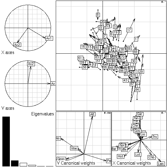Figure 3: Plot of a co-inertia analysis: projection of the principal axes of the two tables (species and environment) on co-inertia axes, eigenvalues screeplot, canonical weights of species and environmental variables, and joint display of the sites.

For each coupling method, a generic plot function allows to represent the various elements required to interpret the results. However, the quality of graphs could vary according to the data set. It is consequently impossible to manage relevant graphical outputs for all cases. That is why these generic plot use graphical functions of ade4 which can be directly called by the user. A brief description of some of these functions is given in table 1.

Function	Objective
`s.arrow`	cloud of points with vectors
`s.chull`	cloud of points with groups by convex hulls
`s.class`	cloud of points with groups by stars or ellipses
`s.corcircle`	correlation circle
`s.distri`	cloud of points with frequency distribution by stars and ellipses
`s.hist`	cloud of points with two marginal histograms
`s.image`	grid of gray-scale rectangles with contour lines
`s.kde2d`	cloud of points with kernel density estimation
`s.label`	cloud of points with labels
`s.logo`	cloud of points with pictures
`s.match`	matching two clouds of points with vectors
`s.traject`	cloud of points with trajectories
`s.value`	cloud of points with numerical variable

Table 1: Objectives of some graphical functions.

Another two-table matching strategy is principal component analyses with respect to instrumental variables (pcaiv, [Rao, 1964]). This approach consists in explaining a triplet (X₂, Q₂, D) by a table of independent variables X₁ and leads to triplet (P_X₁X₂, Q₂,D) where P_X₁=X₁(X₁^tDX₁)^-1X₁^tD. This family of methods are constrained ordinations, among which redundancy analysis [van den Wollenberg, 1977] and canonical correspondence analysis [Ter Braak, 1986] are the most frequently used in ecology. Note that canonical correspondence analysis can also be performed using the cca wrapper function which takes two tables as arguments. The example given below is then exactly equivalent to plot(cca(jv73$poi,jv73$morpho,scannf=FALSE)). While the cca function of ade4 is a particular case of pcaiv, the cca function of the package vegan is a more traditional implementation of the method which could be preferred by ecologists.

 plot(pcaiv(coa1, jv73$morpho, scannf = FALSE))

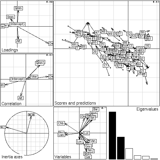Figure 4: Plot of a CCA seen as a particular case of PCAIV: environmental variables loadings and correlations with CCA axes, projection of principal axes on CCA axes, species scores, eigenvalues screeplot, and joint display of the rows of the two tables (position of the sites by averaging (points) and by regression (arrow tips)).

Orthogonal analysis (pcaivortho) allows to remove the effect of independent variables and corresponds to the triplet (P_^X₁X₂, Q₂,D) where P_^X₁=I - P_X₁. Between-class (between) and within-class (within) analyses (see Chessel et al. [2004] for details) are particular cases of PCAIV and orthogonal PCAIV when there is only one categorical variable (i.e. factor) in X₁. Within-class analyses allow to take into account a partition of individuals into groups and focus on structures which are common to all groups. It can be seen as a first step to K-table methods.

 wit1 <- within(coa1, fac = jv73$fac.riv, 
     scannf = FALSE)
 plot(wit1)

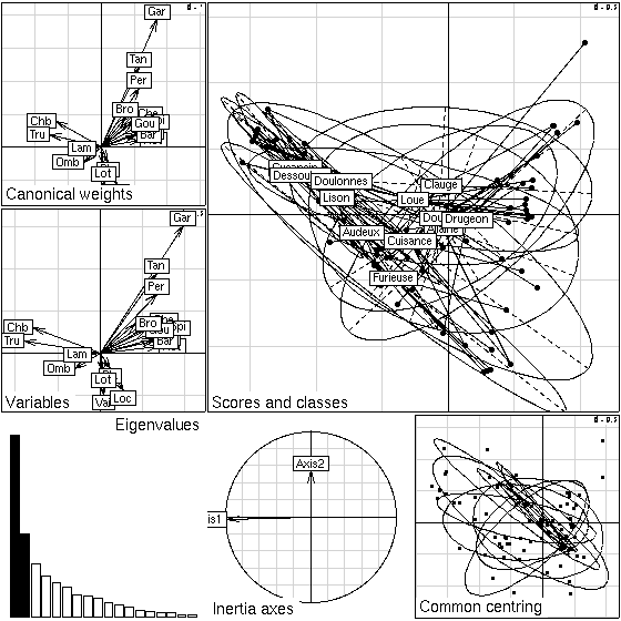Figure 5: Plot of a within-class analysis: species loadings, species scores, eigenvalues screeplot, projection of principal axes on within-class axes, sites scores (common centring), projections of sites and groups (i.e. rivers in this example) on within-class axes.

4 The K-table class

Class ktab corresponds to collections of more than two duality diagrams, which internal structures are to be compared. Three formats of these collections can be considered:

(X₁,Q₁,D), (X₂,Q₂,D),..., (X_K,Q_K,D)
(X₁,Q,D₁), (X₂,Q,D₂),..., (X_K,Q,D_K) stored in the form of (X₁^t,D₁,Q), (X₂^t,D₂,Q),..., (X_K^t,D_K,Q)
(X₁,Q,D), (X₂,Q,D),..., (X_K,Q,D) which can also be stored in the form of (X₁^t,D,Q), (X₂^t,D,Q),..., (X_K^t,D,Q)

Each statistical triplet corresponds to a separate analysis (e.g., principal component analysis, correspondence analysis ...). The common dimension of the K statistical triplets are the rows of tables which can represent individuals (samples, statistical units) or variables. Utilities for building and manipulating ktab objects are available. K-table can be constructed from a list of tables (ktab.list.df), a list of dudi objects (ktab.list.dudi), a within-class analysis (ktab.within) or by splitting a table (ktab.data.frame). Generic functions to transpose (t.ktab), combine (c.ktab) or extract elements ([.ktab) are also available. The sepan function can be used to compute automatically the K separate analyses.

 kt1 <- ktab.within(wit1)
 sep1 <- sepan(kt1)
 kplot.sepan.coa(sep1, permute.row.col = TRUE)

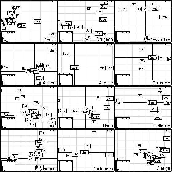Figure 6: Kplot of 12 separate correspondence analyses (same species, different sites).

When the ktab object is built, various statistical methods can be used to analyse it. The foucart function can be used to analyse K tables of positive number having the same rows and the same columns and that can be analysed by a CA [Foucart, 1984,Pavoine et al., 2007]. Partial triadic analysis [Tucker, 1966] is a first step toward three modes principal component analysis [Kroonenberg, 1989] and can be computed with the pta function. It must be used on K triplets having the same row and column weights. The pta function can be used to perform the STATICO method [Simier et al., 1999,Thioulouse et al., 2004]. This allows to analyse a pair of ktab objects which have been combined by the ktab.match2ktabs function.

Multiple factor analysis (mfa, [Escofier and Pagès, 1994]), multiple co-inertia analysis (mcoa, [Chessel and Hanafi, 1996]) and the STATIS method (statis, [Lavit et al., 1994]) can be used to compare K triplets having the same row weights. The STATIS method can also be used to compare K triplets having the same column weights, which is a first step toward Common PCA [Flury, 1988].

 sta1 <- statis(kt1, scannf = F)
 plot(sta1)

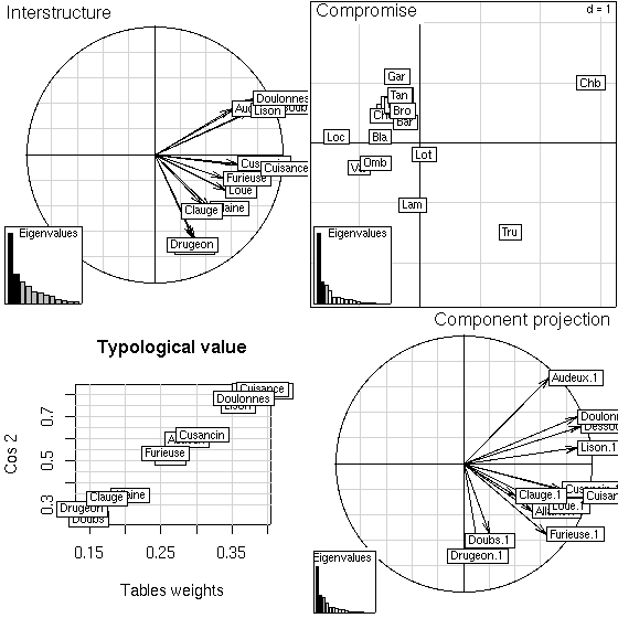Figure 7: Plot of STATIS analysis: interstructure, typological value of each table, compromise and projection of principal axes of separate analyses onto STATIS axes.

The kplot generic function is associated to the foucart, mcoa, mca, pta, sepan, sepan.coa and statis methods, giving adapted collections of graphics.

 kplot(sta1, traj = TRUE, arrow = FALSE, 
     unique = TRUE, clab = 0)

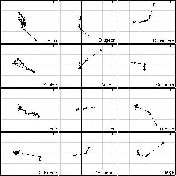Figure 8: Kplot of the projection of the sites of each table on the principal axes of the compromise of STATIS analysis.

5 Conclusion

The ade4 package provides many methods to analyse multivariate ecological data sets. This diversity of tools is a methodological answer to the great variety of questions and data structures associated to biological questions. Specific methods dedicated to the analysis of biodiversity, spatial, genetic or phylogenetic data are also available in the package. The adehabitat brother-package contains tools to analyse habitat selection by animals while the ade4TkGUI package provides a graphical interface to ade4. More ressources can be found on the ade4 website (http://pbil.univ-lyon1.fr/ADE-4/).

Bibliography

[Cazes 1980]: P. Cazes. L'analyse de certains tableaux rectangulaires décomposés en blocs : généralisation des propriétés rencontrées dans l'étude des correspondances multiples. I. Définitions et applications à l'analyse canonique des variables qualitatives. Les Cahiers de l'Analyse des Données, 5: 145-161, 1980.
[Chessel and Hanafi 1996]: D. Chessel and M. Hanafi. Analyse de la co-inertie de K nuages de points. Revue de Statistique Appliquée, 44 (2): 35-60, 1996.
[Chessel et al. 2004]: D. Chessel, A.-B. Dufour, and J. Thioulouse. The ade4 package-I- One-table methods. R News, 4: 5-10, 2004.
[Digby and Kempton 1987]: P. G. N. Digby and R. A. . Kempton. Multivariate Analysis of Ecological Communities. Chapman and Hall, Population and Community Biology Series, London, 1987.
[Dolédec and Chessel 1994]: S. Dolédec and D. Chessel. Co-inertia analysis: an alternative method for studying species-environment relationships. Freshwater Biology, 31: 277-294, 1994.
[Dray and Dufour 2007]: S. Dray and A. Dufour. The ade4 package: implementing the duality diagram for ecologists. Journal of Statistical Software, 22 (4): 1-20, 2007.
[Dray et al. 2003a]: S. Dray, D. Chessel, and J. Thioulouse. Procrustean co-inertia analysis for the linking of multivariate datasets. Ecoscience, 10: 110-119, 2003a.
[Dray et al. 2003b]: S. Dray, D. Chessel, and J. Thioulouse. Co-inertia analysis and the linking of ecological tables. Ecology, 84 (11): 3078-3089, 2003b.
[Escofier and Pagès 1994]: B. Escofier and J. Pagès. Multiple factor analysis (AFMULT package). Computational Statistics and Data Analysis, 18: 121-140, 1994.
[Escoufier 1987]: Y. Escoufier. The duality diagram : a means of better practical applications. In P. Legendre and L. Legendre, editors, Development in numerical ecology, pages 139-156. NATO advanced Institute , Serie G .Springer Verlag, Berlin, 1987.
[Flury 1988]: B. Flury. Common Principal Components and Related Multivariate. models. Wiley and Sons, New-York, 1988.
[Foucart 1984]: T. Foucart. Analyse factorielle de tableaux multiples. Masson, Paris, 1984.
[Goecke 2005]: R. Goecke. 3D lip tracking and co-inertia analysis for improved robustness of audio-video automatic speech recognition. In Proceedings of the Auditory-Visual Speech Processing Workshop AVSP 2005, pages 109-114, 2005.
[Gower 1971]: J. Gower. Statistical methods of comparing different multivariate analyses of the same data. In F. Hodson, D. Kendall, and P. Tautu, editors, Mathematics in the archaeological and historical sciences, pages 138-149. University Press, Edinburgh, 1971.
[Heo and Gabriel 1998]: M. Heo and K. Gabriel. A permutation test of association between configurations by means of the RV coefficient. Communications in Statistics - Simulation and Computation, 27: 843-856, 1998.
[Holmes 2006]: S. Holmes. Multivariate analysis: The French way. In N. D. and S. T., editors, Festschrift for David Freedman. IMS, Beachwood, OH, 2006.
[Jackson 1995]: D. Jackson. PROTEST: a PROcustean randomization TEST of community environment concordance. Ecosciences, 2: 297-303, 1995.
[Kroonenberg 1989]: P. Kroonenberg. The analysis of multiple tables in factorial ecology. iii three-mode principal component analysis:änalyse triadique complète". Acta OEcologica, OEcologia Generalis, 10: 245-256, 1989.
[Lavit et al. 1994]: C. Lavit, Y. Escoufier, R. Sabatier, and P. Traissac. The ACT (STATIS method). Computational Statistics and Data Analysis, 18: 97-119, 1994.
[Mercier et al. 1992]: P. Mercier, D. Chessel, and S. Dolédec. Complete correspondence analysis of an ecological profile data table: a central ordination method. Acta OEcologica, 13: 25-44, 1992.
[Montaña and Greig-Smith 1990]: C. Montaña and P. Greig-Smith. Correspondence analysis of species by environmental variable matrices. Journal of Vegetation Science, 1: 453-460, 1990.
[Pavoine et al. 2007]: S. Pavoine, J. Blondel, M. Baguette, and D. Chessel. A new technique for ordering asymmetrical three-dimensional data sets in ecology. Ecology, 88: 512-523, 2007.
[Rao 1964]: C. Rao. The use and interpretation of principal component analysis in applied research. Sankhya A, 26: 329-359, 1964.
[Simier et al. 1999]: M. Simier, L. Blanc, F. Pellegrin, and D. Nandris. Approche simultanée de K couples de tableaux : application à l'étude des relations pathologie végétale-environment. Revue de Statistique Appliquée, 47: 31-46, 1999.
[Ter Braak 1986]: C. Ter Braak. Canonical correspondence analysis : a new eigenvector technique for multivariate direct gradient analysis. Ecology, 67: 1167-1179, 1986.
[Thioulouse et al. 2004]: J. Thioulouse, M. Simier, and D. Chessel. Simultaneous analysis of a sequence of pairs of ecological tables with the STATICO method. Ecology, 85: 272-283, 2004.
[Tucker 1958]: L. . Tucker. An inter-battery method of factor analysis. Psychometrika, 23: 111-136, 1958.
[Tucker 1966]: L. Tucker. Some mathemetical notes on three-mode factor analysis. Psychometrika, 31: 279-311, 1966.
[van den Wollenberg 1977]: A. van den Wollenberg. Redundancy analysis, an alternative for canonical analysis. Psychometrika, 42 (2): 207-219, 1977.
[Verneaux 1973]: J. Verneaux. Cours d'eau de Franche-Comté (Massif du Jura). Recherches écologiques sur le réseau hydrographique du Doubs. Essai de biotypologie. Thèse de doctorat, Université de Besançon, Besançon, 1973.

File translated from T_EX by T_TH, version 3.78.
On 23 Oct 2007, 18:32.