Summary: Correspondence analysis of codon usage data is a widely used method in sequence analysis, but the variability in amino acid composition between proteins is a confounding factor when one wants to analyse synonymous codon usage variability. A simple and natural way to cope with this problem is to use within-group correspondence analysis. There is, however, no user-friendly implementation of this method available for genomic studies. Our motivation was to provide to the community a Web facility to easily study synonymous codon usage on a subset of data available in public genomic databases.
Availability: Availability through the Pôle Bioinformatique Lyonnais (PBIL) Web server at http://pbil.univ-lyon1.fr/datasets/charif04/ with a demo allowing to reproduce the figure in the present application note. All underlying software is distributed under a GPL licence.
Contact: http://pbil.univ-lyon1.fr/members/lobry/
choosebank(bank = "trypano")
This line selects the data bank in which we want to retrieve the sequences to be analysed. The complete list of the different banks that are accessible is available here. Here the bank trypano is a frozen subset of GenBank: its content is stable to allow for the reproducibility of results. It was build on 27-JAN-2004 from GenBank release 139 by selecting data from Leishamnia major, Trypanosoma brucei and Trypanosoma cruzi. It contains 117,177,046 bases 158,838 sequences 4,744 subsequences and 2,114 references.
The second step is to get all the sequences mnemonics we are interested in. Because we are using the same query for three different species, we define a simple function to avoid code duplication. As input it has two arguments: listname to store the result of the query and species which contains the name of the species of interest.
    myquery <- function(listname, species)
    {
      requested <- paste("SP =", species, "ET O = nuclear ET T = cds ET NO K = partial")
      query(listname, requested)
    }
If we call for instance this function with Leishmania major as second argument, the request will be SP = Leishmania major ET O = nuclear ET T = CDS ET NO K = partial, which means that we want all the sequences from Leishmania major that are from a nuclear origin and that are coding sequences and that are not partial. For a complete description of the query language go there. Now, we have just to call this function with our three species:
    myquery("lm", "Leishmania major")
    myquery("tb", "Trypanosoma brucei")
    myquery("tc", "Trypanosoma cruzi")
The mnemonics of corresponding sequences are stored in lm$req (1,467 sequence names) tb$req (1,772 sequence names) and tc$req (679 sequence names). From them, we can extract the sequences, this is the next step.
For this, we just apply the function getseq to our list of sequences names (they are returned as a vector of chars).
    seqlm <- lapply(lm$req, getSequence)
    seqtb <- lapply(tb$req, getSequence)
    seqtc <- lapply(tc$req, getSequence)
We use the function uco() to compute codon usage for a sequence. We define here a small utility function to put this into a data.frame :
    mkdata <- function(seqs)
    {
      tab <- sapply(seqs, uco)
      tab <- as.data.frame(tab)
      return( tab )
    }
We apply this function to our three species :
    tablm <- mkdata(seqlm)
    tabtb <- mkdata(seqtb)
    tabtc <- mkdata(seqtc)
In this section we want to remove CDS with in-frame stop codons (translated by "*" here) and CDS that have less than 100 codons:
    cleanup <- function(tab)
    {
      aa <- translate(sapply(rownames(tab),s2c))
      tab <- tab[ , colSums(tab[which(aa == "*"), ]) == 1]
      tab <- tab[ , colSums(tab) > 100 ]
      return(tab)
    }

    tablm <- cleanup(tablm) # now 1,427 cds
    tabtb <- cleanup(tabtb) # now 1,298 cds
    tabtc <- cleanup(tabtc) # now   635 cds
Here, we merge the data from the three species and name the columns by their rank:
    tab <- cbind(tablm, tabtb, tabtc)
    names(tab) <- 1:ncol(tab)
We run then simple correpondence analysis, asking to keep automatically two factors:
coa <- dudi.coa(tab, scan = FALSE, nf = 2)
Now, to run synonymous codon usage analysis, we first define a factor, facaa, saying for which amino-acid the codons are coding and then use this factor to run the within analysis:
    facaa <- as.factor(aaa(translate(sapply(rownames(tab),s2c))))
    scua <- wca(coa, facaa, scan = FALSE, nf = 2)
We first define a factor corresponding to the three species under analysis:
    facsp <- as.factor(rep(c("lm","tb","tc"),
                           c(ncol(tablm),ncol(tabtb),ncol(tabtc))))
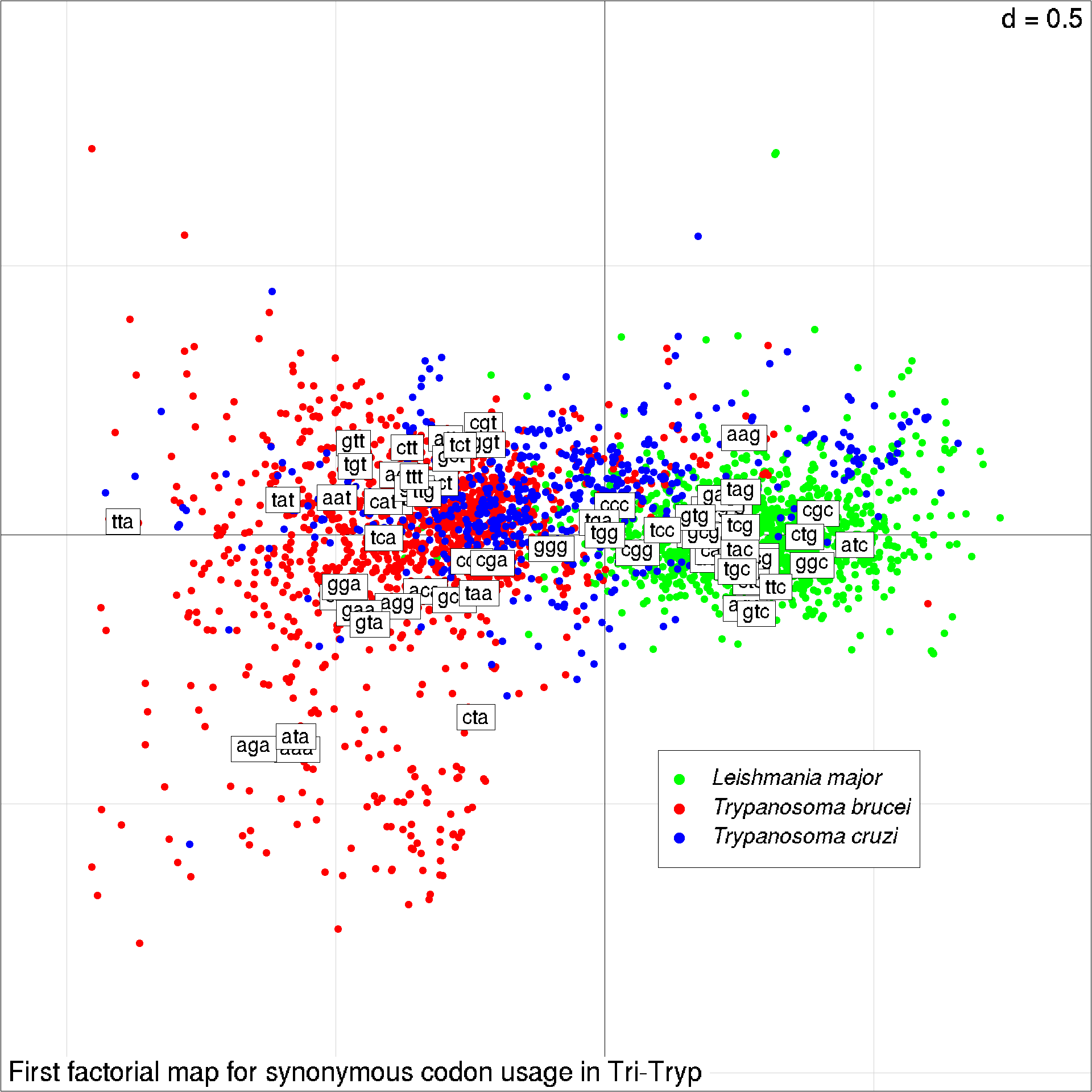
We use then s.class to plot the first factorial map with a color code for the three species:
    s.class(scua$co, fac = facsp, cstar = 0, label = "",
            col = c("green", "red", "blue"), cell=0, cpoint=0.8,
            sub="First factorial map for synonymous codon usage in Tri-Tryp")
We add then the coordinates of colums, that is the codons here, as a label with their names:
s.label(scua$li, add.plot = TRUE, clab = 0.75)
This last line is just to add a legend to the plot:
    legend( x = 0.1, y = -0.4, pch = 19, col = c("green", "red", "blue"),
           legend = c(expression(italic("Leishmania major")),
                      expression(italic("Trypanosoma brucei")),
                      expression(italic("Trypanosoma cruzi"))),
           xjust = 0, cex = 0.8)
If you want to export data in a tabular form, you have first to set up the current working directory as follows:
setwd("/ftp/ftpdir/pub/ADE-User/data")
Then, write the data you want to get, for instance the table of codon counts, tab, in the three species:
write.table(tab, file="tab")
And then download the corresponding file from our ftp server there.
 Back to PBIL home page