Zagordi & Lobry (2005) Gene 347:175

This page allows for the on-line reproduction (and some extras) of the figures in the paper: Zagordi, O., Lobry, J.R. (2005) Forcing reversibility in the no strand-bias substitution model allows for the theoretical and practical identifiability of its 5 parameters from pairwise DNA sequence comparisons. Gene, 347:175-182 [DATASET] [arXiv] [preprint PDF]

Acknowledgements: This contribution partly comes from the thesis Osvaldo Zagordi presented at Naples University in October 2002. The authors thank warmly professor Luca Peliti for connecting them during the strapp 04 meeting (Dresden, Germany, July 5-10 2004). OZ also because he was introduced by him to the beauties of biological systems. They thank Manolo Gouy for kindly providing the multiple alignment of rRNA sequences and for many constructive suggestions. The manuscript was also improved thanks to the comments from three anonymous reviewers.

Abstract: Because of the base pairing rules in DNA, some mutations experienced by a portion of DNA during its evolution result in the same substitution, as we can only observe differences in coupled nucleotides. Then, in the absence of a bias between the two DNA strands, a model with at most 6 different parameters instead of 12 is sufficient to study the evolutionary relationship between homologous sequences derived from a common ancestor. On the other hand the same symmetry reduces the number of independent observations which can be made. Such a reduction can in some cases invalidate the calculation of the parameters. A compromise between biologically acceptable hypotheses and tractability is introduced and a five parameter reversible no-strand-bias condition (RNSB) is presented. The identifiability of the parameters under this model is shown by examples.

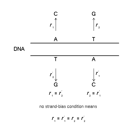
1. The no strand-bias condition

Figure 1 was to explain the no strand-bias condition: If the rates for a certain substitution are the same on both strands of DNA, one can deduce the equivalence of this rate to the one between the complementary bases.

par(no.readonly = TRUE) -> opar
par(mar = rep(0.1, 4))
plot.new()
plot.window(xlim = c(0,1), ylim = c(0,1))

#
# DNA strands:
#
lines(c(0.2, 0.9), c(0.6, 0.6), lwd = 2)
lines(c(0.2, 0.9), c(0.7, 0.7), lwd = 2)
text(0.05, 0.65, "DNA", cex = 1.5, pos = 4)

#
# Top left:
#
text(0.4, 0.7, "A", cex = 1.5, pos = 3)
text(0.4, 0.9, "C", cex = 1.5, pos = 3)
arrows(0.4, 0.8, 0.4, 0.9, le = 0.1)
text(0.4, 0.83, expression(paste(italic(r), scriptstyle(atop(,1)))), cex = 1.5, pos = 2)

#
# Top right:
#
text(0.7, 0.7, "T", cex = 1.5, pos = 3)
text(0.7, 0.9, "G", cex = 1.5, pos = 3)
arrows(0.7, 0.8, 0.7, 0.9, le = 0.1)
text(0.7, 0.83, expression(paste(italic(r), scriptstyle(atop(,2)))), cex = 1.5, pos = 4)

#
# Bottom left:
#
text(0.4, 0.6, "T", cex = 1.5, pos = 1)
text(0.4, 0.4, "G", cex = 1.5, pos = 1)
arrows(0.4, 0.5, 0.4, 0.4, le = 0.1)
text(0.4, 0.44, expression(paste(italic(r), scriptstyle(atop("\'",2)))), cex = 1.5, pos = 2)
text(0.4, 0.3, expression(paste(italic(r), scriptstyle(atop(,1)), " = ", italic(r), scriptstyle(atop("\'",2)))), cex = 1.5)
#
# Bottom right:
#
text(0.7, 0.6, "A", cex = 1.5, pos = 1)
text(0.7, 0.4, "C", cex = 1.5, pos = 1)
arrows(0.7, 0.5, 0.7, 0.4, le = 0.1)
text(0.7, 0.45, expression(paste(italic(r), scriptstyle(atop("\'",1)))), cex = 1.5, pos = 4)
text(0.7, 0.3, expression(paste(italic(r), scriptstyle(atop(,2)), " = ", italic(r), scriptstyle(atop("\'",1)))), cex = 1.5)
#
# Bottom bottom:
#
text(0.5, 0.2, "no strand-bias condition means", cex = 1.2)
text(0.5, 0.1, expression(paste(italic(r), scriptstyle(atop(,1)), " = ", 
               italic(r), scriptstyle(atop("\'",1)), " = ",
               italic(r), scriptstyle(atop(,2)), " = ",
               italic(r), scriptstyle(atop("\'",2)))), cex = 1.5)

par(opar)

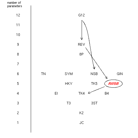
2. The position of the new RNSB model

Figure 2 showed the position of the new RNSB within the hierarchy of already published DNA substitution models. Simplifications leading from a model to a simpler one are indicated by arrows. Only those directly referring to the discussion in the paper were drawn. This figure has been adapted from Robert Schmidt's work.

par(no.readonly = TRUE) -> opar
par(mar = rep(0.1, 4))
plot.new()
plot.window(xlim = c(0,1), ylim = c(0,13))

#
# Number of parameters:
#
for( i in 1:12)
  text(0.1, i, i)
text(0,13,"number of\nparameters", pos=4, cex = 0.8)
lines(c(0.2, 0.2), c(0,13))
#
# Models:
#
text(0.6, 12, "G12")

text(0.6, 9, "REV")

text(0.6, 8, "8P")

text(0.3, 6, "TN")
text(0.5, 6, "SYM")
text(0.7, 6, "NSB")
text(0.9, 6, "GIN")

text(0.5, 5, "HKY")
text(0.7, 5, "TK5")

text(0.4, 4, "EI")
text(0.6, 4, "TK4")
text(0.8, 4, "B4")

text(0.5, 3, "T3")
text(0.7, 3, "3ST")

text(0.6, 2, "K2")
text(0.6, 1, "JC")

#
# RNSB and arrows:
#

text(0.85, 5, expression(bolditalic("RNSB")), col="red")
circle <- function(x,y,rx, ry)
{
  alpha <- seq(from = 0, to = 2*pi, length = 200)
  lines(x + rx*cos(alpha), y + ry*sin(alpha))
}
circle(0.85, 5, 0.07, 0.4)
arrows(0.63, 8.7, 0.8, 5.5, le = 0.1) #REV->RNSB
arrows(0.6, 11.5, 0.6, 9.5, le = 0.1) #G12->REV
arrows(0.78, 4.7, 0.65, 4, le = 0.1) #RNSB->TK4
lines(spline(c(0.6,0.65,0.69,0.7),c(11.5,10,7,6.5), method="natural"))
arrows(0.6998,6.51,0.7,6.5, le=0.1) #G12->NSB

par(opar)

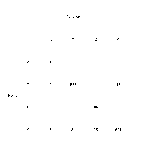
3. Data set: the observed difference matrix

The data set we used is the observed difference matrix between Homo and Xenopus in the multiple alignement of rRNA sequences from Gouy & Li (1989) Nature,339:145-147. The file of aligned sequences in mase format is here. The script is editable so that you can produce data for any available couple of species by changing the values of idx1 and idx2. The list of available species is:

[1]  "Homo"             "Mus"              "Xenopus"          "Drosophila"       
[5]  "Caenorhabditis"   "Oryza"            "Lycopersicon"     "Citrus"           
[9]  "Saccharomyces"    "Prorocentrum"     "Tetrahymena"      "Dictyostelium"    
[13] "Physarum"         "Crithidia"        "Methanococcus"    "Methanobacterium" 
[17] "Desulfurococcus"  "Sulfolobus"       "Thermoproteus"    "Thermoplasma"     
[21] "Halococcus"       "HalobacteriumH"   "HalobacteriumM"   "Escherichia"      
[25] "Pseudomonas"      "Rhodobacter"      "BacillusSubt"     "BacillusStea"     
[29] "Micrococcus"      "Streptomyces"     "Pirellula"        "Anacystis"        
[33] "EuglenaCP"        "Ruminobacter"     "Leptospira"       "Thermus"

#
# Select a couple of species (1 is Homo, 3 is Xenopus):
#

idx1 <- 1
idx2 <- 3

#
# Load library seqinr to read the alignment file:
#

#library(seqinr) preloaded on the server, not usefull here
read.alignment("/www/htdocs/members/lobry/repro/gene05/lsufrags.mase", "mase") -> data

#
# Print available species in dataset:
#

print(data$nam)

#
# Get aligned sequences as a vector of chars in lower case:
#

seq1 <- tolower(s2c(data$seq[idx1]))
seq2 <- tolower(s2c(data$seq[idx2]))

#
# Get species names:
#

sp1 <- data$nam[idx1]
sp2 <- data$nam[idx2]

#
# Counts of nucleotide differences (substitutions) between sequences:
#

naa <- sum( seq1 == "a" & seq2 == "a" )
nat <- sum( seq1 == "a" & seq2 == "t" )
nac <- sum( seq1 == "a" & seq2 == "c" )
nag <- sum( seq1 == "a" & seq2 == "g" )

nta <- sum( seq1 == "t" & seq2 == "a" )
ntt <- sum( seq1 == "t" & seq2 == "t" )
ntc <- sum( seq1 == "t" & seq2 == "c" )
ntg <- sum( seq1 == "t" & seq2 == "g" )

nca <- sum( seq1 == "c" & seq2 == "a" )
nct <- sum( seq1 == "c" & seq2 == "t" )
ncc <- sum( seq1 == "c" & seq2 == "c" )
ncg <- sum( seq1 == "c" & seq2 == "g" )

nga <- sum( seq1 == "g" & seq2 == "a" )
ngt <- sum( seq1 == "g" & seq2 == "t" )
ngc <- sum( seq1 == "g" & seq2 == "c" )
ngg <- sum( seq1 == "g" & seq2 == "g" )

#
# print observed nucleotide difference (substitution) matrix:
#

print("In seq2: A T C G")
print(paste("A:", naa, nat, nac, nag))
print(paste("T:", nta, ntt, ntc, ntg))
print(paste("C:", nca, nct, ncc, ncg))
print(paste("G:", nga, ngt, ngc, ngg))

#
# Make a Latex table for the paper:
#

cat("% --- Table of observed nucleotide differences ---\n")
cat("\\begin{tabular}{l l l l l l}\n")
cat("\\hline \\hline\n")
cat(paste("& & \\multicolumn{4}{c}{", sp2, "}\\\\\n"))
cat("\\hline\n")
cat("& & A & T & C & G\\\\\n")
cat(paste("& A &", naa, "&", nat, "&", nac, "&", nag , "\\\\\n")) 
cat(paste(sp1, "& T &", nta, "&", ntt, "&", ntc, "&", ntg , "\\\\\n")) 
cat(paste("& C &", nca, "&", nct, "&", ncc, "&", ncg , "\\\\\n")) 
cat(paste("& G &", nga, "&", ngt, "&", ngc, "&", ngg , "\\\\\n")) 
cat("\\hline \\hline\n")
cat("\\end{tabular}\n")
cat("% ------------------------------------------------\n")

#
# Show the table as an R graphics:
#

par(no.readonly = TRUE) -> opar
par(mar = rep(0.1, 4))
plot.new()
plot.window(xlim = c(0, 6), ylim = c(0, 6))

#
# Lines:
#
lines(c(0,6), c(6,6))
lines(c(0,6), c(5.95,5.95))
lines(c(0,6), c(5, 5))
lines(c(0,6), c(0,0))
lines(c(0,6), c(0.05,0.05))
#
# Species names:
#
text(3, 5.5, sp2)
text(0, 2, sp1, pos = 4)
#
# Bases
#
text(2, 4.5, "A")
text(3, 4.5, "T")
text(4, 4.5, "G")
text(5, 4.5, "C")

text(1, 3.5, "A")
text(1, 2.5, "T")
text(1, 1.5, "G")
text(1, 0.5, "C")
#
# Data (base counts)
#
text(2, 3.5, naa)
text(3, 3.5, nat)
text(4, 3.5, nag)
text(5, 3.5, nac)

text(2, 2.5, nta)
text(3, 2.5, ntt)
text(4, 2.5, ntg)
text(5, 2.5, ntc)

text(2, 1.5, nga)
text(3, 1.5, ngt)
text(4, 1.5, ngg)
text(5, 1.5, ngc)

text(2, 0.5, nca)
text(3, 0.5, nct)
text(4, 0.5, ncg)
text(5, 0.5, ncc)

par(opar)

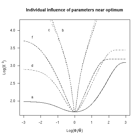
4. Individual influence of parameters near optimum

We used the chi-squared as an adjustement criterion and then used non-linear minimization to get an estimate of parameter values. Figure 3 showed the shape of the chi-squared criterion when parameter values are changed one at once around the minimum. Here are the parameter values you should obtain in the case of the Homo versus Xenopus comparison:

Minimum : 48.80783 at:
a  = 0.00174775040817750 
b  = 0.0112180666689986 
c  = 0.0155821726728541 
d  = 0.00486598075643191 
f  = 0.0163616450505670

#
# Select a couple of species (1 is Homo, 3 is Xenopus):
#

idx1 <- 1
idx2 <- 3

#
# Load library seqinr to read the alignment file:
#

#library(seqinr) # preloaded on our server, not usefull in this context

read.alignment("/www/htdocs/members/lobry/repro/gene05/lsufrags.mase", "mase") -> data

#
# Print available species in dataset:
#

print(data$nam)

#
# Get aligned sequences as a vector of chars in lower case:
#

seq1 <- tolower(s2c(data$seq[idx1]))
seq2 <- tolower(s2c(data$seq[idx2]))

#
# Get species names:
#

sp1 <- data$nam[idx1]
sp2 <- data$nam[idx2]

#
# Counts of nucleotide differences (substitutions) between sequences:
#

naa <- sum( seq1 == "a" & seq2 == "a" )
nat <- sum( seq1 == "a" & seq2 == "t" )
nac <- sum( seq1 == "a" & seq2 == "c" )
nag <- sum( seq1 == "a" & seq2 == "g" )

nta <- sum( seq1 == "t" & seq2 == "a" )
ntt <- sum( seq1 == "t" & seq2 == "t" )
ntc <- sum( seq1 == "t" & seq2 == "c" )
ntg <- sum( seq1 == "t" & seq2 == "g" )

nca <- sum( seq1 == "c" & seq2 == "a" )
nct <- sum( seq1 == "c" & seq2 == "t" )
ncc <- sum( seq1 == "c" & seq2 == "c" )
ncg <- sum( seq1 == "c" & seq2 == "g" )

nga <- sum( seq1 == "g" & seq2 == "a" )
ngt <- sum( seq1 == "g" & seq2 == "t" )
ngc <- sum( seq1 == "g" & seq2 == "c" )
ngg <- sum( seq1 == "g" & seq2 == "g" )

#
# print observed nucleotide difference (substitution) matrix:
#

print("In seq2: A T C G")
print(paste("A:", naa, nat, nac, nag))
print(paste("T:", nta, ntt, ntc, ntg))
print(paste("C:", nca, nct, ncc, ncg))
print(paste("G:", nga, ngt, ngc, ngg))

#
# Make a Latex table for the paper:
#

mktable <- function() {
 cat("% --- Table of observed nucleotide differences ---\n")
 cat("\\begin{tabular}{l l l l l l}\n")
 cat("\\hline \\hline\n")
 cat(paste("& & \\multicolumn{4}{c}{", sp2, "}\\\\\n"))
 cat("\\hline\n")
 cat("& & A & T & C & G\\\\\n")
 cat(paste("& A &", naa, "&", nat, "&", nac, "&", nag , "\\\\\n")) 
 cat(paste(sp1, "& T &", nta, "&", ntt, "&", ntc, "&", ntg , "\\\\\n")) 
 cat(paste("& C &", nca, "&", nct, "&", ncc, "&", ncg , "\\\\\n")) 
 cat(paste("& G &", nga, "&", ngt, "&", ngc, "&", ngg , "\\\\\n")) 
 cat("\\hline \\hline\n")
 cat("\\end{tabular}\n")
 cat("% ------------------------------------------------\n")
}
mktable()

#
# Total number of observations is n:
#

n = ngg + nga + ngt + ngc +
    nag + naa + nat + nac +
    ntg + nta + ntt + ntc +
    ncg + nca + nct + ncc

#
# xnn for normalized entries :
#

xaa <- naa/n
xac <- nac/n
xag <- nag/n
xat <- nat/n

xca <- nca/n
xcc <- ncc/n
xcg <- ncg/n
xct <- nct/n

xga <- nga/n
xgc <- ngc/n
xgg <- ngg/n
xgt <- ngt/n

xta <- nta/n
xtc <- ntc/n
xtg <- ntg/n
xtt <- ntt/n

#
# Define this just for compatibility with C code:
#
Power <- function(x, y)
{
  return( x^y )
}
E <- exp(1)
Sqrt <- sqrt

#
# Simple function just to debug:
#
show.me <- function(x)
{
  print(paste(deparse(substitute(x)), "=", x))
}

#
#  This is the function to minimize. At best it can be zero, so we can have an idea of how good is our estimate of the
#  model. xac, xag etc are the observed entries of the divergence matrix. This should be enough for the minimization to run:
#  chisquare as a function of a,...,f. Of we are right running a minimization looking for all the six parameters should fail,
#  whereas enforcing e = cd/b should work.
#

stuff <- function(t = 1, a = 1.001, b = 1.002 , c = 1.003, d = 1.004, f = 1.006, verbose = FALSE)
{

#
# Enforce reversibility here, supplied values for parameter e are not
# taken into account:
#

e = c*d/b

#
# This is no more needed in the present version, but I keep it
# for the record as a comment:
#
#  fequil = 0.5*(b+d)/(b+c+d+e);
#

Xplus = ((b + d)*((b + d)/(b + c + d + e) + (1 - (b + d)/(b + c + d + e))/Power(E,2*(b + c + d + e)*t)))/(b + c + d + e);
  
  Yplus = (1 - (b + d)/(b + c + d + e))*(1 - (b + d)/(b + c + d + e) + (b + d)/((b + c + d + e)*Power(E,2*(b + c + d + e)*t)));
  
  Zplus = (2*(b + d)*(1 - (b + d)/(b + c + d + e))*(1 - Power(E,-2*(b + c + d + e)*t)))/(b + c + d + e);
  
  Xminus = (2*(b - d)*(((b + d)*(c - e))/(b + c + d + e) - (b - d)*(1 - (b + d)/(b + c + d + e)))*Power(E,(-2*a - b - c - d - e - 2*f)*t) + 
     Power(E,(-2*a - b - c - d - e - 2*f - Sqrt(4*(b - d)*(c - e) + Power(-2*a + b - c + d - e + 2*f,2)))*t)*
      (Power(b - d,2)*(1 - (b + d)/(b + c + d + e)) + 
        ((b + d)*((b - d)*(c - e) + ((-2*a + b - c + d - e + 2*f)*
                (-2*a + b - c + d - e + 2*f - Sqrt(4*(b - d)*(c - e) + Power(-2*a + b - c + d - e + 2*f,2))))/2.))/(b + c + d + e))
       + Power(E,(-2*a - b - c - d - e - 2*f + Sqrt(4*(b - d)*(c - e) + Power(-2*a + b - c + d - e + 2*f,2)))*t)*
      (Power(b - d,2)*(1 - (b + d)/(b + c + d + e)) + 
        ((b + d)*((b - d)*(c - e) + ((-2*a + b - c + d - e + 2*f)*
                (-2*a + b - c + d - e + 2*f + Sqrt(4*(b - d)*(c - e) + Power(-2*a + b - c + d - e + 2*f,2))))/2.))/(b + c + d + e))
	    )/(4*(b - d)*(c - e) + Power(-2*a + b - c + d - e + 2*f,2));
  
  Yminus = (-2*(c - e)*(((b + d)*(c - e))/(b + c + d + e) - (b - d)*(1 - (b + d)/(b + c + d + e)))*Power(E,(-2*a - b - c - d - e - 2*f)*t) + 
	    Power(E,(-2*a - b - c - d - e - 2*f + Sqrt(4*(b - d)*(c - e) + Power(-2*a + b - c + d - e + 2*f,2)))*t)*
	    (((b + d)*Power(c - e,2))/(b + c + d + e) + (1 - (b + d)/(b + c + d + e))*
	     ((b - d)*(c - e) + ((-2*a + b - c + d - e + 2*f)*
				 (-2*a + b - c + d - e + 2*f - Sqrt(4*(b - d)*(c - e) + Power(-2*a + b - c + d - e + 2*f,2))))/2.)) + 
	    Power(E,(-2*a - b - c - d - e - 2*f - Sqrt(4*(b - d)*(c - e) + Power(-2*a + b - c + d - e + 2*f,2)))*t)*
	    (((b + d)*Power(c - e,2))/(b + c + d + e) + (1 - (b + d)/(b + c + d + e))*
	     ((b - d)*(c - e) + ((-2*a + b - c + d - e + 2*f)*
				 (-2*a + b - c + d - e + 2*f + Sqrt(4*(b - d)*(c - e) + Power(-2*a + b - c + d - e + 2*f,2))))/2.)))/
    (4*(b - d)*(c - e) + Power(-2*a + b - c + d - e + 2*f,2));
  
  Zminus =(-2*(((b + d)*(c - e))/(b + c + d + e) - (b - d)*(1 - (b + d)/(b + c + d + e)))*Power(E,(-2*a - b - c - d - e - 2*f)*t)*
      (-2*a + b - c + d - e + 2*f) + Power(E,(-2*a - b - c - d - e - 2*f + 
          Sqrt(4*(b - d)*(c - e) + Power(-2*a + b - c + d - e + 2*f,2)))*t)*
      (-((b - d)*(1 - (b + d)/(b + c + d + e))*(-2*a + b - c + d - e + 2*f - 
             Sqrt(4*(b - d)*(c - e) + Power(-2*a + b - c + d - e + 2*f,2)))) + 
        ((b + d)*(c - e)*(-2*a + b - c + d - e + 2*f + Sqrt(4*(b - d)*(c - e) + Power(-2*a + b - c + d - e + 2*f,2))))/
         (b + c + d + e)) + Power(E,(-2*a - b - c - d - e - 2*f - Sqrt(4*(b - d)*(c - e) + Power(-2*a + b - c + d - e + 2*f,2)))*
        t)*(((b + d)*(c - e)*(-2*a + b - c + d - e + 2*f - Sqrt(4*(b - d)*(c - e) + Power(-2*a + b - c + d - e + 2*f,2))))/
         (b + c + d + e) - (b - d)*(1 - (b + d)/(b + c + d + e))*
	    (-2*a + b - c + d - e + 2*f + Sqrt(4*(b - d)*(c - e) + Power(-2*a + b - c + d - e + 2*f,2)))))/
    (4*(b - d)*(c - e) + Power(-2*a + b - c + d - e + 2*f,2));
     
  S1 = (Xplus + Xminus)/4;
     
  S2 = (Yplus + Yminus)/4;
     
  Q1 = (Xplus - Xminus)/4;
     
  Q2 = (Yplus - Yminus)/4;
     
  P = (Zplus + Zminus)/8; # <------ I have changed the denominator from 4 to 8
     
  R = (Zplus - Zminus)/8; # <------ I have changed the denominator from 4 to 8

#
# Alternative expression (with the chisquare <- n*chisquare
# 
# chisquare = (xag*xag + xga*xga + xtc*xtc + xct*xct)/P + (xac*xac + xca*xca + xtg*xtg + xgt*xgt)/R + (xat*xat + xta*xta)/Q1 +
#   (xcg*xcg + xgc*xgc)/Q2 + (xaa*xaa + xtt*xtt)/S1 + (xcc*xcc + xgg*xgg)/S2 - 1;

newchisquare = ( (n*P - nag)^2 + (n*P - nga)^2 + (n*P - ntc)^2 + (n*P - nct)^2 )/(n*P) +
                 ( (n*R - nac)^2 + (n*R - nca)^2 + (n*R - ntg)^2 + (n*R - ngt)^2 )/(n*R) +
                 ( (n*Q1 - nat)^2 + (n*Q1 - nta)^2 )/(n*Q1) +
                 ( (n*Q2 - ncg)^2 + (n*Q2 - ngc)^2 )/(n*Q2) +
                 ( (n*S1 - naa)^2 + (n*S1 - ntt)^2 )/(n*S1) +
                 ( (n*S2 - ncc)^2 + (n*S2 - ngg)^2 )/(n*S2)
  
  if(verbose)
  {
    show.me(t)
    show.me(a)
    show.me(b)
    show.me(c)
    show.me(d)
    show.me(e)
    show.me(f)
    show.me(n)
    show.me(Xplus)
    show.me(Yplus)
    show.me(Zplus)
    show.me(Xminus)
    show.me(Yminus)
    show.me(Zminus)
    show.me(S1)
    show.me(S2)
    show.me(Q1)
    show.me(Q2)
    show.me(P)
    show.me(R)
    show.me(4*P + 4*R + 2*Q1 + 2*Q2 + 2*S1 + 2*S2)
    show.me(chisquare)
    show.me(newchisquare)
    show.me(n*chisquare)
  }
  return( newchisquare )
}

#
# paramter estimate: constrained estimation so that parameters are always
# positive
#

objf <- function(p)
{
  return(stuff(t=1, a = 10^(p[1]), b = 10^(p[2]), c = 10^p[3], d = 10^p[4], f = 10^p[5]))
}

pguess <- c(10^-2.7, 10^-2, 10^-1.8, 10^-2.3, 10^-1.8)

#
# This is the function for nonlinear minimisation:
#

nlm(f = objf, p = pguess) -> nlmtry

#
# Print results:
#
print(nlmtry)
hatp <- 10^nlmtry$estimate

print(paste("a  =", hatp[1]))
print(paste("b  =", hatp[2]))
print(paste("c  =", hatp[3]))
print(paste("d  =", hatp[4]))
print(paste("f  =", hatp[5]))

#
# Compute the chisquare for a bad model in which each entry is set to the mean n/16,
# just to get an idea of maximum acceptable value and scale graphs.
#

maxchisquare = ( (n/16 - nag)^2 + (n/16 - nga)^2 + (n/16 - ntc)^2 + (n/16 - nct)^2 )/(n/16) +
                 ( (n/16 - nac)^2 + (n/16 - nca)^2 + (n/16 - ntg)^2 + (n/16 - ngt)^2 )/(n/16) +
                 ( (n/16 - nat)^2 + (n/16 - nta)^2 )/(n/16) +
                 ( (n/16 - ncg)^2 + (n/16 - ngc)^2 )/(n/16) +
                 ( (n/16 - naa)^2 + (n/16 - ntt)^2 )/(n/16) +
                 ( (n/16 - ncc)^2 + (n/16 - ngg)^2 )/(n/16)
#
# save gaphical parameter settings
#

par(no.readonly = TRUE) -> oldpar
par( mar = 1.1*par("mar")) #increase marges of plot
#
# See a
#

chimin <- nlmtry$minimum
fracp <- 10^seq(from = -3, to = 3, length = 300) # Fraction of paramter value in log scale

hata <- hatp[1]
ya <- sapply(hata*fracp, function(x) { stuff(a = x, b = hatp[2], c = hatp[3], d = hatp[4], f = hatp[5])})
plot(x = log10(fracp), y = log10(ya), 
  xlab = expression(Log(Theta/hat(Theta))), 
  ylim = c(log10(chimin), log10(2*maxchisquare)),
   ylab = expression(Log(italic(Chi)^{~~2})), las = 1, type = "l", lty = 1,
  main = "Individual influence of parameters near optimum")
  
#abline(h = log10(maxchisquare), lty = 2)
text(-2.5, 2.1, "a")

#
# See b
# 
hatb <- hatp[2]
yb <- sapply(hatb*fracp, function(x) { stuff(a = hatp[1], b = x, c = hatp[3], d = hatp[4], f = hatp[5])})
lines(log10(fracp), log10(yb), lty = 2)
text(-0.7, 4, "b")

#
# See c
# 
hatc <- hatp[3]
yc <- sapply(hatc*fracp, function(x) { stuff(a = hatp[1], b = hatp[2], c = x, d = hatp[4], f = hatp[5])})
lines(log10(fracp), log10(yc), lty = 3)
text(-1.5, 4, "c")

#
# See d
#

hatd <- hatp[4]
yd <- sapply(hatd*fracp, function(x) { stuff(a = hatp[1], b = hatp[2], c = hatp[3], d = x, f = hatp[5])})
lines(log10(fracp), log10(yd), lty = 4)
text(-2.5, 3, "d")

#
# See f
#

hatf <- hatp[5]
yf <- sapply(hatf*fracp, function(x) { stuff(a = hatp[1], b = hatp[2], c = hatp[3], d = hatp[4], f = x)})
lines(log10(fracp), log10(yf), lty = 5)
text(-2.5, 3.8, "f")

#
# Restore gaphical parameter settings:
#

par(oldpar)

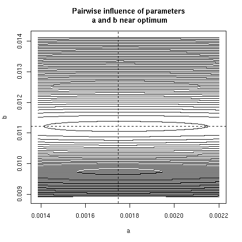
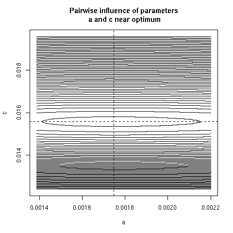
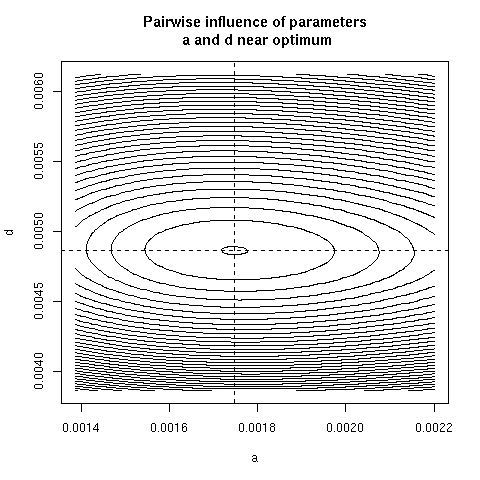
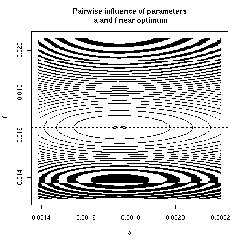
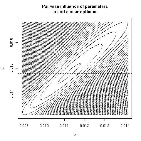
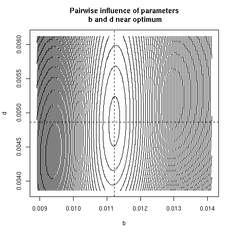
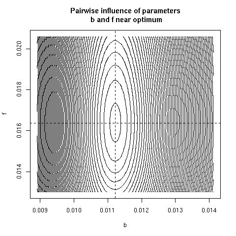
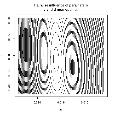
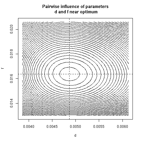
5. Paiwise influence of parameters near optimum

We have explored systematically the shape of the Chi-squared criterion for all pairs of paramters around the minimum. In the paper we showed only (Figure 4) the case of the (b, c) pair because it was the unique instance for which a structural correlation was found. Here, all parameter pairs are given.

If you have any problems or comments, please contact Jean Lobry.