ade4 dans
Analyses des Données Ecologiques : méthodes Exploratoires et Euclidiennes en sciences de l'Environnement

Article Rnews 2004

The ade4 package - I : One-table methods

by Daniel Chessel, Anne B Dufour and Jean Thioulouse

Chessel, D., A.-B. Dufour, and J. Thioulouse. 2004. The ade4 package-I- One-table methods. R News 4:5-10.

Introduction
The duality diagram class
Distance matrices
Taking into account groups of individuals
Permutation tests
Conclusion

1 Introduction

This paper is a short summary of the main classes defined in the ade4 package for one table analysis methods (e.g., principal component analysis). Other papers will detail the classes defined in ade4 for two-tables coupling methods (such as canonical correspondence analysis, redundancy analysis, and co-inertia analysis), for methods dealing with K-tables analysis (i.e., three-ways tables), and for graphical methods.

This package is a complete rewrite of the ADE4 software ([Thioulouse et al., 1997], http://pbil.univ-lyon1.fr/ADE-4/) for the R environment. It contains Data Analysis functions to analyse Ecological and Environmental data in the framework of Euclidean Exploratory methods, hence the name ade4 (i.e., 4 is not a version number but means that there are four E in the acronym). The ade4 package is available in CRAN, but it can also be used directly online, thanks to the Rweb system (http://pbil.univ-lyon1.fr/Rweb/). This possibility is being used to provide multivariate analysis services in the field of bioinformatics, particularly for sequence and genome structure analysis at the PBIL (http://pbil.univ-lyon1.fr/). An example of these services is the automated analysis of the codon usage of a set of DNA sequences by correspondence analysis ([Perrière et al., 2003] http://pbil.univ-lyon1.fr/mva/coa.php).

2 The duality diagram class

The basic tool in ade4 is the duality diagram [Escoufier, 1987]. A duality diagram is simply a list that contains a triplet (X, Q, D): - X is a table with n rows and p columns, considered as p points in Rⁿ (column vectors) or n points in R^p (row vectors). - Q is a p ×p diagonal matrix containing the weights of the p columns of X, and used as a scalar product in R^p (Q is stored under the form of a vector of length p). - D is a n ×n diagonal matrix containing the weights of the n rows of X, and used as a scalar product in Rⁿ (D is stored under the form of a vector of length n). For example, if X is a table containing normalized quantitative variables, if Q is the identity matrix I_p and if D is equal to [1/n]I_n, the triplet corresponds to a principal component analysis on correlation matrix (normed PCA). Each basic method corresponds to a particular triplet (see table 1), but more complex methods can also be represented by their duality diagram.

Functions	Analyses	Notes
dudi.pca	principal component	1
dudi.coa	correspondence	2
dudi.acm	multiple correspondence	3
dudi.fca	fuzzy correspondence	4
dudi.mix	analysis of a mixture of numeric and factors	5
dudi.nsc	non symmetric correspondence	6
dudi.dec	decentered correspondence	7

The dudi functions. 1: Principal component analysis, same as prcomp/princomp. 2: Correspondence analysis [Greenacre, 1984]. 3: Multiple correspondence analysis [Tenenhaus and Young, 1985]. 4: Fuzzy correspondence analysis [Chevenet et al., 1994]. 5: Analysis of a mixture of numeric variables and factors [Hill and Smith, 1976], [Kiers, 1994]. 6: Non symmetric correspondence analysis [Kroonenberg and Lombardo, 1999]. 7: Decentered correspondence analysis [Dolédec et al., 1995].

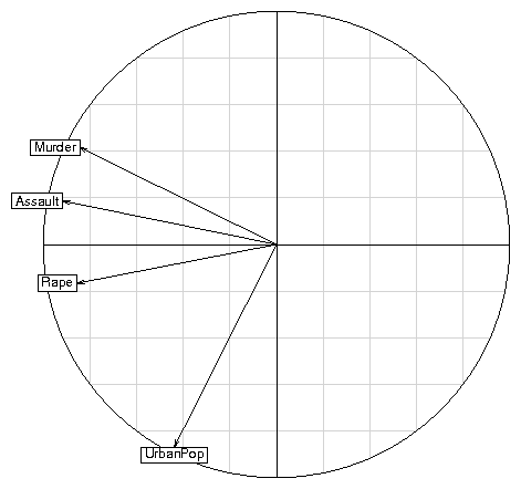
The singular value decomposition of a triplet gives principal axes, principal components, and row and column coordinates, which are added to the triplet for later use.

We can use for example a well-known dataset from the base package :

 data(USArrests)
 pca1 <- dudi.pca(USArrests, scannf = FALSE, nf = 3)

scannf = FALSE means that the number of principal components that will be used to compute row and column coordinates should not be asked interactively to the user, but taken as the value of argument nf (by default, nf = 2). Other parameters allow to choose between centered, normed or raw PCA (default is centered and normed), and to set arbitrary row and column weights. The pca1 object is a duality diagram, i.e., a list made of several vectors and dataframes:

 pca1

Duality diagramm
class: pca dudi
$call: dudi.pca(df = USArrests, scannf = FALSE, nf = 3)

$nf: 3 axis-components saved
$rank: 4
eigen values: 2.48 0.9898 0.3566 0.1734
  vector length mode    content       
1 $cw    4      numeric column weights
2 $lw    50     numeric row weights   
3 $eig   4      numeric eigen values  

  data.frame nrow ncol content             
1 $tab       50   4    modified array      
2 $li        50   3    row coordinates     
3 $l1        50   3    row normed scores   
4 $co        4    3    column coordinates  
5 $c1        4    3    column normed scores
other elements: cent norm

pca1$lw and pca1$cw are the row and column weights that define the duality diagram, together with the data table (pca1$tab). pca1$eig contains the eigenvalues. The row and column coordinates are stored in pca1$li and pca1$co. The variance of these coordinates is equal to the corresponding eigenvalue, and unit variance coordinates are stored in pca1$l1 and pca1$c1 (this is usefull to draw biplots).

The general optimization theorems of data analysis take particular meanings for each type of analysis, and graphical functions are proposed to draw the canonical graphs, i.e., the graphical expression corresponding to the mathematical property of the object. For example, the normed PCA of a quantitative variable table gives a score that maximizes the sum of squared correlations with variables. The PCA canonical graph is therefore a graph showing how the sum of squared correlations is maximized for the variables of the data set. On the USArrests example, we obtain the following graphs:

 score(pca1)

 s.corcircle(pca1$co)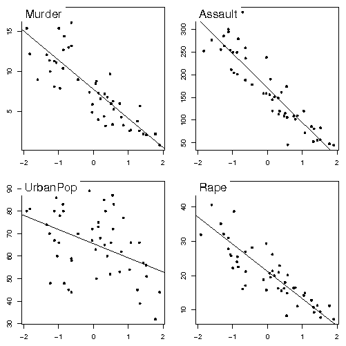

Figure 1: One dimensional canonical graph for a normed PCA. Variables are displayed as a function of row scores, to get a picture of the maximization of the sum of squared correlations.

Figure 2: Two dimensional canonical graph for a normed PCA (correlation circle): the direction and length of arrows show the quality of the correlation between variables and between variables and principal components.

The scatter function draws the biplot of the PCA (i.e., a graph with both rows and columns superimposed):

 scatter(pca1)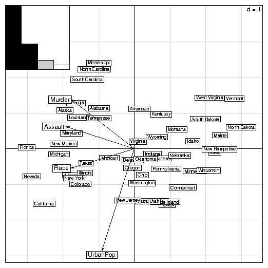

Figure 3: The PCA biplot. Variables are symbolized by arrows and they are superimposed to the individuals display. The scale of the graph is given by a grid, which size is given in the upper right corner. Here, the length of the side of grid squares is equal to one. The eigenvalues bar chart is drawn in the upper left corner, with the two black bars corresponding to the two axes used to draw the biplot. Grey bars correspond to axes that were kept in the analysis, but not used to draw the graph.

Separate factor maps can be drawn with the s.corcircle (see figure 2) and s.label functions:

 s.label(pca1$li)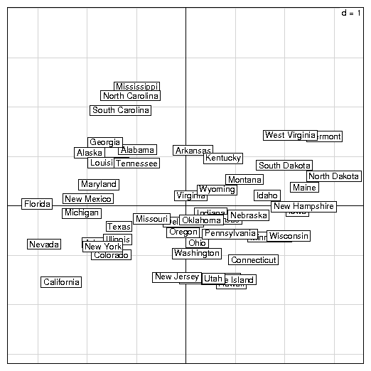

Figure 4: Individuals factor map in a normed PCA.

3 Distance matrices

A duality diagram can also come from a distance matrix, if this matrix is Euclidean (i.e., if the distances in the matrix are the distances between some points in a Euclidean space). The ade4 package contains functions to compute dissimilarity matrices (dist.binary for binary data, and dist.prop for frequency data), test whether they are Euclidean [Gower and Legendre, 1986], and make them Euclidean (quasieuclid, lingoes, [Lingoes, 1971], cailliez, [Cailliez, 1983]). These functions are useful to ecologists who use the works of [Legendre and Anderson, 1999] and [Legendre and Legendre, 1998].

The Yanomama data set ([Manly, 1991]) contains three distance matrices between 19 villages of Yanomama Indians. The dudi.pco function can be used to compute a principal coordinates analysis (PCO, [Gower, 1966]), that gives a Euclidean representation of the 19 villages. This Euclidean representation allows to compare the geographical, genetic and anthropometric distances.

 data(yanomama)
 gen <- quasieuclid(as.dist(yanomama$gen))
 geo <- quasieuclid(as.dist(yanomama$geo))
 ant <- quasieuclid(as.dist(yanomama$ant))
 geo1 <- dudi.pco(geo, scann = FALSE, nf = 3)
 gen1 <- dudi.pco(gen, scann = FALSE, nf = 3)
 ant1 <- dudi.pco(ant, scann = FALSE, nf = 3)
 par(mfrow = c(2, 2))
 scatter(geo1)
 scatter(gen1)
 scatter(ant1, posi = "bottom")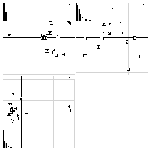

Figure 5: Comparison of the PCO analysis of the three distance matrices of the Yanomama data set: geographic, genetic and anthropometric distances.

4 Taking into account groups of individuals

In sites x species tables, rows correspond to sites, columns correspond to species, and the values are the number of individuals of species j found at site i. These tables can have many columns and cannot be used in a discriminant analysis. In this case, between-class analyses (between function) are a better alternative, and they can be used with any duality diagram. The between-class analysis of triplet (X, Q, D) for a given factor f is the analysis of the triplet (G, Q, D_w), where G is the table of the means of table X for the groups defined by f, and D_w is the diagonal matrix of group weights. For example, a between-class correspondence analysis (BCA) is very simply obtained after a correspondence analysis (CA):

 data(meaudret)
 coa1 <- dudi.coa(meaudret$fau, scannf = FALSE)
 bet1 <- between(coa1, meaudret$plan$sta, scannf = FALSE)
 plot(bet1)

The meaudret$fau dataframe is an ecological table with 24 rows corresponding to six sampling sites along a small French stream (the Meaudret). These six sampling sites were sampled four times (spring, summer, winter and autumn), hence the 24 rows. The 13 columns correspond to 13 ephemerotera species. The CA of this data table is done with the dudi.coa function, giving the coa1 duality diagram. The corresponding bewteen-class analysis is done with the between function, considering the sites as classes (meaudret$plan$sta is a factor defining the classes). Therefore, this is a between-sites analysis, which aim is to discriminate the sites, given the distribution of ephemeroptera species. This gives the bet1 duality diagram, and Figure 6 shows the graph obtained by plotting this object.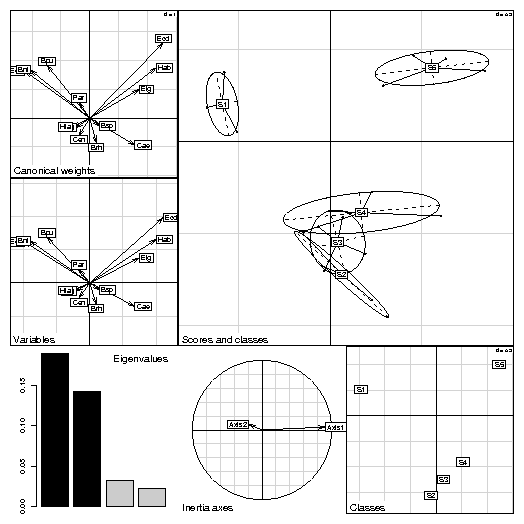

Figure 6: BCA plot. This is a composed plot, made of : 1- the species canonical weights (top left), 2- the species scores (middle left), 3- the eigenvalues bar chart (bottom left), 4- the plot of plain CA axes projected into BCA (bottom center), 5- the gravity centers of classes (bottom right), 6- the projection of the rows with ellipses and gravity center of classes (main graph).

Like between-class analyses, linear discriminant analysis (discrimin function) can be extended to any duality diagram (G,(X^tDX)^-,D_w), where (X^tDX)^- is a generalized inverse. This gives for example a correspondence discriminant analysis ([Perrière et al., 1996], [Perrière and Thioulouse, 2002]), that can be computed with the discrimin.coa function. Opposite to between-class analyses are within-class analyses, corresponding to diagrams (X-YD^-1_wY^tDX, Q, D) (within functions). These analyses extend to any type of variables the Multiple Group Principal Component Analysis (MGPCA, [Thorpe, 1983a], [Thorpe, 1983b], [Thorpe and Leamy, 1983]. Furthermore, the within.coa function introduces the double within-class correspondence analysis (also named internal correspondence analysis, [Cazes et al., 1988]).

5 Permutation tests

Permutation tests (also called Monte-Carlo tests, or randomization tests) can be used to assess the statistical significance of between-class analyses. Many permutation tests are available in the ade4 package, for example mantel.randtest, procuste.randtest, randtest.between, randtest.coinertia, RV.rtest, randtest.discrimin, and several of these tests are available both in R (mantel.rtest) and in C (mantel.randtest) programming langage. The R version allows to see how computations are performed, and to write easily other tests, while the C version is needed for performance reasons.

The statistical significance of the BCA can be evaluated with the randtest.between function. By default, 999 permutations are simulated, and the resulting object (test1) can be plotted (Figure 7). The p-value is highly significant, which confirms the existence of differences between sampling sites. The plot shows that the observed value is very far to the right of the histogram of simulated values.

 test1 <- randtest.between(bet1)
 test1

Monte-Carlo test
Call: randtest.between(xtest = bet1)

Observation: 0.4292 

Based on 999 replicates
Simulated p-value: 0.001 
Alternative hypothesis: greater 

    Std.Obs Expectation    Variance 
   3.834237    0.256985    0.002018

 plot(test1, main = "Between class inertia")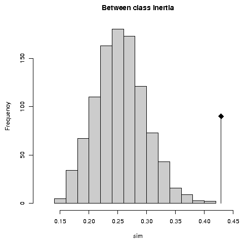

Figure 7: Histogram of the 999 simulated values of the randomization test of the bet1 BCA. The observed value is given by the vertical line, at the right of the histogram.

6 Conclusion

We have described only the most basic functions of the ade4 package, considering only the simplest one-table data analysis methods. Many other dudi methods are available in ade4, for example multiple correspondence analysis (dudi.acm), fuzzy correspondence analysis (dudi.fca), analysis of a mixture of numeric variables and factors (dudi.mix), non symmetric correspondence analysis (dudi.nsc), decentered correspondence analysis (dudi.dec).

We are preparing a second paper, dealing with two-tables coupling methods, among which canonical correspondence analysis and redundancy analysis are the most frequently used in ecology ([Legendre and Legendre, 1998]). The ade4 package proposes an alternative to these methods, based on the co-inertia criterion ([Dray et al., 2003]).

The third category of data analysis methods available in ade4 are K-tables analysis methods, that try to extract the stable part in a series of tables. These methods come from the STATIS strategy, [Lavit et al., 1994] (statis and pta functions) or from the multiple coinertia strategy (mcoa function). The mfa and foucart functions perform two variants of K-tables analysis, and the STATICO method (function ktab.match2ktabs, [Thioulouse et al., 2004]) allows to extract the stable part of species-environment relationships, in time or in space.

Methods taking into account spatial constraints (multispati function) and phylogenetic constraints (phylog function) are under development.

Bibliography

[Cailliez, 1983]: Cailliez, F. (1983). The analytical solution of the additive constant problem. Psychometrika, 48:305-310.
[Cazes et al., 1988]: Cazes, P., Chessel, D., and Dolédec, S. (1988). L'analyse des correspondances internes d'un tableau partitionné : son usage en hydrobiologie. Revue de Statistique Appliquée, 36:39-54.
[Chevenet et al., 1994]: Chevenet, F., Dolédec, S., and Chessel, D. (1994). A fuzzy coding approach for the analysis of long-term ecological data. Freshwater Biology, 31:295-309.
[Dolédec et al., 1995]: Dolédec, S., Chessel, D., and Olivier, J. (1995). L'analyse des correspondances décentrée: application aux peuplements ichtyologiques du haut-rhône. Bulletin Français de la Pêche et de la Pisciculture, 336:29-40.
[Dray et al., 2003]: Dray, S., Chessel, D., and Thioulouse, J. (2003). Co-inertia analysis and the linking of ecological tables. Ecology, 84:3078-3089.
[Escoufier, 1987]: Escoufier, Y. (1987). The duality diagramm : a means of better practical applications. In Legendre, P. and Legendre, L., editors, Development in numerical ecology, pages 139-156. NATO advanced Institute , Serie G .Springer Verlag, Berlin.
[Gower, 1966]: Gower, J. (1966). Some distance properties of latent root and vector methods used in multivariate analysis. Biometrika, 53:325-338.
[Gower and Legendre, 1986]: Gower, J. and Legendre, P. (1986). Metric and euclidean properties of dissimilarity coefficients. Journal of Classification, 3:5-48.
[Greenacre, 1984]: Greenacre, M. (1984). Theory and applications of correspondence analysis. Academic Press, London.
[Hill and Smith, 1976]: Hill, M. and Smith, A. (1976). Principal component analysis of taxonomic data with multi-state discrete characters. Taxon, 25:249-255.
[Kiers, 1994]: Kiers, H. (1994). Simple structure in component analysis techniques for mixtures of qualitative ans quantitative variables. Psychometrika, 56:197-212.
[Kroonenberg and Lombardo, 1999]: Kroonenberg, P. and Lombardo, R. (1999). Nonsymmetric correspondence analysis: a tool for analysing contingency tables with a dependence structure. Multivariate Behavioral Research, 34:367-396.
[Lavit et al., 1994]: Lavit, C., Escoufier, Y., Sabatier, R., and Traissac, P. (1994). The act (statis method). Computational Statistics and Data Analysis, 18:97-119.
[Legendre and Anderson, 1999]: Legendre, P. and Anderson, M. (1999). Distance-based redundancy analysis: testing multispecies responses in multifactorial ecological experiments. Ecological Monographs, 69:1-24.
[Legendre and Legendre, 1998]: Legendre, P. and Legendre, L. (1998). Numerical ecology. Elsevier Science BV, Amsterdam, 2nd english edition edition.
[Lingoes, 1971]: Lingoes, J. (1971). Somme boundary conditions for a monotone analysis of symmetric matrices. Psychometrika, 36:195-203.
[Manly, 1991]: Manly, B. F. J. (1991). Randomization and Monte Carlo methods in biology. Chapman and Hall, London.
[Perrière et al., 2003]: Perrière, G., Combet, C., Penel, S., Blanchet, C., Thioulouse, J., Geourjon, C., Grassot, J., Charavay, C., Gouy, M. Duret, L., and Deléage, G. (2003). Integrated databanks access and sequence/structure analysis services at the pbil. Nucleic Acids Research, 31:3393-3399.
[Perrière et al., 1996]: Perrière, G., Lobry, J., and Thioulouse, J. (1996). Correspondence discriminant analysis: a multivariate method for comparing classes of protein and nucleic acid sequences. Computer Applications in the Biosciences, 12:519-524.
[Perrière and Thioulouse, 2002]: Perrière, G. and Thioulouse, J. (2002). Use of correspondence discriminant analysis to predict the subcellular location of bacterial proteins. Computer Methods and Programs in Biomedicine, in press.
[Tenenhaus and Young, 1985]: Tenenhaus, M. and Young, F. (1985). An analysis and synthesis of multiple correspondence analysis, optimal scaling, dual scaling, homogeneity analysis ans other methods for quantifying categorical multivariate data. Psychometrika, 50:91-119.
[Thioulouse et al., 1997]: Thioulouse, J., Chessel, D., Dolédec, S., and Olivier, J. (1997). Ade-4: a multivariate analysis and graphical display software. Statistics and Computing, 7:75-83.
[Thioulouse et al., 2004]: Thioulouse, J., Simier, M., and Chessel, D. (2004). Simultaneous analysis of a sequence of paired ecological tables. Ecology, 85:272-283.
[Thorpe, 1983a]: Thorpe, R. S. (1983a). A biometric study of the effects of growth on the analysis of geographic variation: Tooth number in green geckos (reptilia: Phelsuma). Journal of Zoology, 201:13-26.
[Thorpe, 1983b]: Thorpe, R. S. (1983b). A review of the numerical methods for recognising and analysing racial differentiation. In Felsenstein, J., editor, Numerical Taxonomy, Series G, pages 404-423. Springer-Verlag, New York.
[Thorpe and Leamy, 1983]: Thorpe, R. S. and Leamy, L. (1983). Morphometric studies in inbred house mice (mus sp.): Multivariate analysis of size and shape. Journal of Zoology, 199:421-432.

File translated from T_EX by T_TH, version 3.67.
On 4 Oct 2006, 14:33.